Digital Twin Based Machining Condition Optimization for CNC Machining Center
Article information
Abstract
Optimization of machining conditions is important in determining productivity and machining quality. This study proposes a method for optimizing the machining conditions of a machine tool using a digital twin of a commercial machine tool comprising physical models of a controller, feed drive systems, and cutting load. The digital twin is constructed and evaluated based on machining experiments, and a genetic algorithm is adopted to determine the machining conditions to minimize the machining time and production cost. The optimal feed rate and spindle speed are obtained for each line of the part program when the cutting force is limited. The machining results demonstrate the effectiveness of the proposed method. After optimization for maximizing the machining speed, the machining time decreased by 16.9%. Similarly, after optimization for minimizing the production cost, the production cost reduced by 36.4%.
1 Introduction
In the machining process, the use of optimal machining conditions is an important factor for increasing machining efficiency [1,2]. In general, machining conditions are generated using computer-aided manufacturing (CAM), considering the shape and material of the product and optimized by skilled workers based on several experiments. However, the series of experiments conducted in the optimization process is time-consuming and increases the production cost.
Model-based machining condition optimization techniques have been proposed to solve this problem. In these methods, a model for predicting machining states such as the cutting force or material removal rate (MRR) is constructed and utilized to derive optimal machining conditions. Model-based optimization methods can save time and cost in experiments because optimal machining conditions are derived in a virtual environment. However, the reliability of optimal conditions depends on the accuracy of the model. Three modeling approaches have been proposed: statistical models, theoretical models, and the integration of theoretical models and machine dynamics.
A statistical model was derived from a large amount of experimental data. Various regression analysis models have been utilized to estimate the relationships between machining conditions and process outcomes, such as surface roughness, tool wear, and production cost [3–8]. Azizi et al. proposed a machining condition optimization method for minimizing surface roughness during turning. A regression model was developed by applying statistical analysis of variance (ANOVA). A statistical model was developed to predict the surface roughness in accordance with the cutting speed, feed rate, depth of cut, and hardness of materials [3]. Manna et al. proposed a machining condition optimization method for minimizing the surface roughness and production cost in turning. A regression model was developed using the Taguchi method and ANOVA. A statistical model was developed for predicting the surface roughness of the workpiece and production cost in accordance with the cutting speed, feed rate, and depth of cut [4]. Sangwan et al. proposed a machining condition optimization method for minimizing surface roughness. A regression model was developed using artificial neural network (ANN). A statistical model for predicting the surface roughness based on the cutting speed, feed rate, and depth of cut was developed. A genetic algorithm was integrated with a neural network model to determine optimal machining conditions [5].
However, such methods require numerous experiments to gather machining data for modeling. Time and money are wasted during this process. The theoretical model is derived from the physical model of machine tool parts and cutting theory. Various theoretical models have been utilized to estimate the relationships between machining conditions and calculated values, such as the MRR and cutting force [9–12]. In contrast to a statistical model, a small amount of machining data is required to identify the model parameters. Meng et al. proposed a machining condition optimization method to minimize the production cost and time in turning. Orthogonal cutting and Taylor tool life models were utilized to estimate the cutting force and tool life, respectively, under various machining conditions developed for optimization [9]. Park et al. proposed a machining condition optimization method to reduce machining time during milling. A model was developed to estimate the MRR and cutting force using the part program. A genetic algorithm was used to determine the optimal feed rate to maintain a cutting force lower than the predetermined cutting force [10].
In the abovementioned study, the dynamic characteristics of the machine tool were not considered when deriving the theoretical models. However, the characteristics of machine tool components, such as the controller and feed drives, play an important role in machining performance. To improve the accuracy of the model, the integration of the theoretical model and machine dynamics, called a digital twin, has been proposed [13–15]. Altintas et al. proposed a machining condition optimization method to reduce machining time using a virtual simulation model. The cutting process and machine dynamic models were integrated. The machining condition was optimized to reduce machining time by considering constraints such as chatter stability, spindle torque, and chip thickness [16]. Lee et al. developed a simulation model to determine the machining conditions for minimizing the energy consumption during milling. A simulation model of the controller, feed drives, auxiliaries, and cutting process was integrated, and the model parameters were identified based on the data obtained from the machining experiments. A genetic algorithm was used to optimize machining conditions [17]. In the aforementioned studies, models were derived using a self-constructed lab-scale machine tool. However, it is difficult to construct a digital twin for a commercial machine tool because detailed information on machine tool components, such as the motor and controller, is not available. Therefore, it is difficult to apply the proposed method to commercial machine tools.
This study proposes a method for optimizing machining conditions by constructing and employing a digital twin of mathematical models of machine tool parts, such as controllers, feed drive systems, and spindles. A cutting-force model was developed to predict the cutting forces based on the position and rotation speed of the tool. A series of experiments was performed to identify the parameters of the controller, feed-drive, and cutting-force models. The digital twin was constructed by combining these models, and then, it was verified experimentally. Genetic algorithm was used to derive the optimal machining conditions that minimized the processing time and production cost without exceeding the predetermined cutting force. Machining experiments were performed to verify whether the optimal machining conditions could achieve the purposes of the optimization.
The remainder of this paper is organized as follows. Section 2 describes the process of constructing a digital twin, including the feed-drive, controller, and cutting-force models. Section 3 describes the process of deriving optimal machining conditions for various purposes using s based on verified digital twins. Finally, Section 4 summarizes the conclusions.
2 Construction of Digital Twin
Fig. 1 shows the experimental apparatus and machining system used in this study. A commercial vertical three-axis machining center (DNM 4500, DN Solutions) with 11 kW of power in the spindle motor and a maximum rotation speed of 8,000 revolutions per minute (RPM) was used as the experimental apparatus. A tool dynamometer (9257B, Kistler) with a sensitivity of −7.93 pC/N and a data acquisition system (NI cDAQ-9179 with NI 9215, National Instruments) were used for measuring X- and Y-axes cutting force. FANUC Servo Guide software was used to obtain the driving currents of the feed drives.
Experimental setup of 3-axis vertical machining center
2.1 Composition of Digital Twin
Fig. 2 shows the composition of the digital twin. It consists of a controller, feed drive system, and cutting-force models that reflect a real machine tool. The digital twin estimates the information of the machine tool and machining process, such as the tool trajectory and cutting load, from the machining conditions and G-code. In addition, process variables such as machining time and production cost were estimated using a digital twin for optimization.
Composition of the digital twin of the commercial 3-axis vertical machining center
2.2 Modeling of Feed Drive Model
To predict the driving information of the feed drive system, it was modeled as follows, considering the inertia, friction force, and cutting force occurring during operation [18].
Ms, x, u, Ff, and Fd are the equivalent loads of the feed drive system, position of the table, driving force, friction force, and cutting force, respectively. Atc, kt, and Lb are the controller torque command, torque constant of the servo motor, and lead length of the feed drive system ball screw, respectively, and the driving force was obtained after measuring the torque command of the motor through the FANUC Servo Guide program. The Stribeck curve model is used to predict the frictional force generated during driving.
Fc, Fs, vs, and μv are the coulomb friction force, maximum static friction force, Stribeck velocity, and viscous friction coefficient, respectively. The four friction force model parameters were derived using a genetic algorithm after measuring the Stribeck curve of the actual feed drive systems [19]. The feed drive system was reciprocated at various speeds, the controller torque command was measured in the constant-speed feed section, and the driving force was calculated. If there was no disturbance, the driving force in the constant-velocity feed section was equal to the friction force. The Stribeck curve was obtained using the driving force at various speeds, and four friction force model parameters were derived using a genetic algorithm. The fitness function of the genetic algorithm is set as follows:
where,
NS, FSS and F̂SS are the number of data points in the Stribeck curve, the measured friction force, and the estimated friction force, respectively. When running the genetic algorithm, the maximum number of evolutions was set to 500 and the fitness limit was set to 100. Because the friction force characteristics differed depending on the direction of the feed axis, the Stribeck curves for each feed direction were measured, and the friction force model parameters were derived. Fig. 3 compares the measured Stribeck curves and those estimated using Eq. (3). Table 1 lists the identified parameters of the feed-drive Stribeck curves.
Comparison of the estimated and measured Stribeck curves: (a) X axis, (b) Y axis, and (c) Z axis
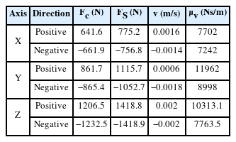
Feed drive model parameters
2.3 Modeling of Controller Model
The controller model is composed of a numerical control kernel (NCK) model that generates the target position of each axis from the G-code input by the user, and a motion control unit (MCU) model that controls the actual feed drive system to follow the target position.
The NCK model consists of an interpreter, interpolator, and velocity profiler. The interpreter interprets the G-code to classify the driving command of the feed axis and spindle and stores the command values, such as the target position and speed of each axis, and the target rotation speed of the spindle in a matrix. The interpolator generates the target speed according to the time of each axis and spindle, based on the command value stored in the matrix. Advanced control functions included in commercial controllers, such as motion blending and look-ahead control for simultaneous multi-axis control, were also applied to the interpolator model by referring to the published controller manual. The interpolator parameters can be set and applied in the same manner as those of a commercial controller. In the velocity profiler, an acceleration/deceleration section is added to the target velocity generated by the interpolator and integrated to generate the final position profile for each axis. The variables used to determine the shape and size of the acceleration/deceleration section are the same as those used in the commercial controller.
Fig. 4 shows the MCU algorithm used in the digital twin model. The MCU performs feedback control in real-time using the position profile generated by the NCK and the position of the feed drive system. The commercial controller used in this study consists of position and speed control loops. In the position control loop, the velocity command is generated by the propositional control of the difference between the reference and actual positions of the feed drive system. In the velocity control loop, the torque command is generated by proportional-integral control of the difference between the velocity command and the actual velocity. However, the torque command estimated by the controller model was significantly different from that estimated by the commercial controller, even though the reference position and feedback values were the same. This is because the commercial controller contains several additional algorithms for data processing, which are not completely introduced in the manual. To solve this problem, the scale factors Spp, SVP, and SVI were multiplied by Pp, Vp, and VI, respectively, to reflect controller performance. Appropriate scale factors were determined by conducting feed experiments at various speeds and using the FANUC Servo Guide program to measure the torque commands and subsequent errors. A genetic algorithm was employed to derive the scale factors for each gain, considering the torque commands and the error values from the actual and modeled systems at various speeds. The fitness function applied in the genetic algorithm was as follows:
Motion control unit algorithm
where
NG, e, ê, Atc, and Âtc were the numbers of data points used in the genetic algorithm, measured following error, predicted following error, measured torque command, and predicted torque command, respectively. When running the genetic algorithm, the maximum number of evolutions was set to 100 and the fitness limit was set to 10. The accuracy of the controller and feed drive models are evaluated by comparing the position control performance with the real feed drives. Figs. 5(a)–(c) show the position and the following error of each axis during reciprocal motion at various velocities. The results show that the proposed models reflect the real system accurately.
Comparison of the position and the following errors of the proposed model and real feed drives: (a) X axis, (b) Y axis, and (c) Z axis
2.4 Modeling of Cutting Load Model
In this study, an orthogonal cutting model was used to derive the x- and y-directional cutting forces and loads [20]. To accelerate the simulation, the helix angle and tool wear were ignored. The model is expressed as follows:
where
Here, Fx, and Fy are the cutting force in the x and y axes, Δx and Δy, and are the changes in the position of the tool center in the x and y directions. Ncut, d, and φj are the number of cutting edges of the tool, the axial cutting depth, and the rotation angle of the jth cutting edge, respectively. Kt, and Ke are the cutting coefficients determined by the type of cutting tool and workpiece material, respectively. g(φj) is a function of the state of the jth cutting edge and can be expressed as follows:
φst, and φex are the start and end angles of the cutting edge, respectively. The cutting load can be calculated as follows:
The cutting coefficients were derived using a genetic algorithm based on the cutting force measured using a tool dynamometer. The fitness function of the genetic algorithm is set as follows:
where
Here NC, Fcf, and F̂cf are the numbers of data points used in the genetic algorithm, measured cutting force, and predicted cutting force, respectively. The maximum number of evolutions was set to 500, and the fitness function limit value was set to 1. Cutting coefficients (Kt = 1.23 × 10⁹ N/m2, and Ke = 0.50) were derived by applying a genetic algorithm to the cutting force measured during slot milling using a machine tool. The material used in the experiments was A6061 aluminum alloy. Note that a 6-mm diameter, 2-flute solid carbide tool (X-POWERS, YG1) was used in all experiments.
2.5 Verification of the Digital Twin
A digital twin was constructed by integrating the controller, feed drive, and cutting load models. The accuracy was verified through machining experiments. Information on the machine tool and machining process estimated by the digital twin was compared with that of a real machine tool for the same G-code and machining conditions. The materials and tools used were the same as those described in Section 2.4. Fig. 6(a) shows the tool path and machining conditions recommended by the tool manufacturer. Fig. 6(b) presents the comparison results of the measured and estimated values for the position and the following errors. Fig. 6(c) shows a comparison of the measured and estimated values for the cutting loads. Table 2 presents the root mean square (RMS) values for each axis following error, and cutting load. The reason for the significant difference in the Z-axis compared to other axes is that this study did not consider control functionality to mitigate the effects of gravity, given the vertical movement characteristics of the Z-axis. The results demonstrate that the digital twin can predict the movements and cutting loads of a real machine tool with high accuracy.
Verification of the digital twin: (a) Tool path, (b) Position and following error, and (c) Cutting load
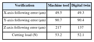
RMS values of the position, following error (F.E.), and cutting load
3 Machining Condition Optimization
Fig. 7 shows the machining condition optimization algorithm utilizing a genetic algorithm and digital twin. The digital twin predicts the movement of the machine tool, cutting load, and process variables included in the optimization fitness function based on the input G-code and computes the fitness value. The evolutionary process is carried out as follows. Individuals are selected based on the predetermined population size. Breeding occurs according to the designated crossover rate, while introducing mutations to prevent convergence towards local minima. Fitness values are extracted by computing them using the digital twin model. Successive generations replace each other as per the specified generation gap. During this process, maximum and minimum values for spindle speed and feed rate are determined, considering equipment performance and machining capability. Following the predefined evolutionary rules, the feed rate and spindle rotation speed were altered, and the modified values were input into the digital twin to calculate the fitness value for the evolved generation. If the fitness value reached the set target, the evolution was terminated, and the feed rate and spindle rotation speed in the final generation were used to modify the original G-code.
Machining condition optimization algorithm
A cutting load limit was set to prevent tool wear and breakage. If the predicted cutting load from the digital twin exceeded this limit, the difference was multiplied by a weigh and added to the fitness function. To verify the effectiveness of the proposed algorithm, optimal machining conditions, which are key process variables that determine productivity, were derived to minimize the machining time and cost. Machining experiments were performed before and after optimization, and the results were compared to demonstrate the improvements achieved using the proposed optimization algorithm. Prior to optimization, machining was conducted under the same conditions as those described in Section 2.5.
3.1 Machining Time Optimization
To minimize machining time, the fitness function of the optimization algorithm was set based on machining time. To prevent breakage of the tool, the cutting load limit was set to 60 N. The fitness function for machining time optimization, Jmt, is set by considering the simulated machining time and cutting load, which is calculated using Eq. (17)
Num(Dt), ss, ff, Ts, Fcf, and Flim represent the number of simulation data points, spindle rotation speed, feed rate, sampling time, model cutting load, cutting load limit, and weight, respectively. The maximum number of evolutions was set to 10, and the fitness function limit was set to 10 for the optimization algorithm. The feed rate was set to evolve within the range between 100 mm/min and 500 mm/min, considering the performance of the machine tool. Similarly, the spindle rotation speed was optimized in the range between 1000 RPM and 8000 RPM. Figs. 8(a) and 8(b) show the G-codes before and after optimization. When the optimized code was applied, the machining time decreased by approximately 16.9%, from 29.48 s to 24.51 s. The surface roughness of the machined surface of the specimen was measured and the Ra values for the codes before and after optimization were 1.78 μm and 1.80 μm, respectively, indicating no significant difference.
Optimized machining conditions: (a) before optimization, (b) after optimization for (b) machining time reduction, and (c) production cost reduction
3.2 Production Cost Optimization
To minimize production cost, the fitness function was set based on the production cost. The cutting force limit was set to 60 N to prevent breakage of the cutting tool. The fitness function for production cost optimization, Jpc, is set by considering the production cost and cutting load, which is calculated using Eq. (18).
Cp represents the production cost, which was calculated as follows:
Here, Ct and Cm are the tool and cutting costs, respectively. Tp, Tl, Pt, Tc, Ep, and Cd are the machining time, tool life, tool price, tool change time, labor cost, and depreciation of the equipment, respectively. The tool price was based on the actual price of the tools used in the experiment, and the labor cost was based on the 2022 minimum wage in South Korea. The depreciation of the equipment was calculated based on its assumed lifespan. The tool life was calculated using the Taylor tool-life equation.
V is the cutting speed calculated using the spindle rotation speed. C, n are coefficients related to the material of the workpiece, tool, cutting fluid, etc., and are set based on a cutting handbook. Table 3 lists the values of the variables used in the cost model. The feed rate was set to evolve within the range of 100 mm/min to 500 mm/min, considering the performance of the machine tool. Similarly, the optimal spindle rotation speed was derived in the range between 1000 RPM and 8000 RPM. Fig. 8(c) shows the G-code after cost optimization, and when the optimized code was applied, the production cost decreased by approximately 36.4% from 120.1 KRW to 76.4 KRW. The surface roughness of the machined surface of the specimen was measured and the Ra values for the codes before and after optimization were 1.78 μm and 1.69 μm, respectively, indicating no significant difference.
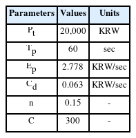
Parameters of the production cost model
4 Conclusion
This study proposed a method to derive the optimal machining conditions primarily for reducing machining time and production costs using digital twins comprising commercial machine tools for milling operations. To this end, a digital twin of the machine tool was developed by integrating individual models of the machine tool components, and it was verified by comparing the estimated values with real data acquired during the machining process. A machining condition optimization algorithm was developed that simulated a G-code using the digital twin. Subsequently, the optimal machining conditions were derived using a genetic algorithm. After the optimal machining conditions for minimizing the processing time were derived and applied to a commercial machine tool, the machining time decreased from 29.48 s to 24.51 s. Additionally, the optimal machining conditions for minimizing production cost were derived and applied to the machine tool, and it resulted in a decrease in production costs from 120.1 KRW to 76.4 KRW. In both optimization results, the cutting loads generated during machining did not exceed the set limit for the cutting load. This confirms that the proposed optimization method can derive optimal machining conditions within a range that does not compromise tool life.
Future works
In process optimization, variations in spindle speed have a significant impact on the occurrence of chatter [20]. Failure to select the appropriate spindle speed can result in chatter, adversely affecting the machining quality. Future research aims to enhance the accuracy of the model and incorporate a chatter prediction model into the digital twin model. This will lead to the development of a more precise digital twin model for machine tools.
Acknowledgement(s)
This work was supported in part by the Korea Institute of Machinery and Materials for the project, Development of Technology for Mobile Platform-based Machining System (No. NK210B) and in part by Korea Institute for Advancement of Technology (KIAT) grant funded by the Korea Government (MOTIE) (P0020616, The Competency Development Program for Industry Specialist).
References
Biography

Beomsik Sim is a Ph.D. student in the Department of Mechanical Engineering, Chungnam National University, Daejeon, South Korea. His research interest is intelligent CNC.

Wonkyun Lee is an Associate Professor in the School of Mechanical Engineering, Chungnam National University, Daejeon, South Korea. He received his B.S. and Ph.D. degrees in Mechanical Engineering in 2008 and 2015, respectively, from Yonsei University, Seoul, South Korea. His research interests include smart machine tool, robotic machining systems and digital twin.