Designable Data Augmentation-based Domain-adaptive Design of Electric Vehicle Considering Dynamic Responses
Article information
Abstract
To address environmental pollution problems, electric vehicles (EVs) are attracting attention as future mobility vehicles. However, an increase in the number of advanced systems coupled with such vehicles imposes a limit on the development of EVs. The conventional design methods require a large amount of experimental and simulation data to satisfy the target performance of the system. Therefore, it takes time to arrive at the desired design solution. Hence, we propose a new design method using domain-adaptive designable data augmentation (DADDA). DADDA is a deep learning-based generative model that applies an inverse generator and domain adaptation concept to the data augmentation algorithm. This model aims to rapidly provide a design solution for a new system with a performance level similar to that of the existing system by adapting the domain of the existing system when the design information for a new system is insufficient.
1 Introduction
Electric vehicles (EVs) are attracting attention as future mobility vehicles, in response to concerns regarding fossil fuel depletion, accelerated global warming, and deepening environmental pollution. Various studies on EV development have been conducted worldwide [1–3]. Most internal EV systems are powered by electricity. Combining existing systems (e.g., transmission, power train, and suspension) of a vehicle with advanced systems (e.g., electronic control units, motors, and batteries) increases the system complexity [4]. Therefore, there is a limit to the development of EV based on conventional design methods. In addition, a newly developed EV requires numerous validations to maximize driving performance and ensure safety. As a conventional design method, design optimization [5,6] has been widely used to optimize the system performance. However, for increasing the reliability of the optimization results, the accuracy of the metamodel is important [7]. Therefore, it is necessary to obtain metamodel data through numerous experiments or simulations. It takes a significant amount of time and cost to extract the experimental or simulation data. Therefore, it is difficult to follow a conventional design method to develop a system, and thus, a new design method is required.
In this paper, we propose a new design method using domain-adaptive designable data augmentation (DADDA). DADDA is a deep learning-based generative model that applies an inverse generator [8] and domain adaptation [9] to data augmentation algorithms, such as generative adversarial networks (GAN). In recent years, to solve the data deficiency problem, GAN, which can generate virtual data similar to actual data, has been presented in many research studies [10–12]. While there have been recent approaches in the domain adaptation [13,14] dealing with fundamental areas of image/signal processing, the present study focuses on both domain adaptation and data augmentation in the electric vehicle design. However, GAN generates only virtual data that are similar to actual data. If the factors affecting the generated virtual data are known, the algorithm can serve as a metamodel. The objective of DADDA is to rapidly provide a design solution for a new system (i.e., target) with a performance level similar to that of the existing system (i.e., source). Furthermore, DADDA can generate virtual target responses using actual source responses and estimate the target design variables that affect the generated virtual target responses. Thus, even if the design data of the target are insufficient, it is possible to design it by referring to the source. The design process using DADDA consists of four steps, as illustrated in Fig. 1. First, the source and target responses are acquired through experiments or simulations. The source had a large number of responses, and the target had a small number of responses. Second, the inverse generator is pre-trained using a small number of design variables and responses acquired from the target to construct a regression network. Thus, it is possible to construct an inverse generator that can output the estimated target design variables when the virtual target responses are inputted into the inverse generator. Third, the training of DADDA proceeds. In this case, DADDA is trained to generate virtual target responses using actual source responses as the training data. Finally, the virtual target responses and design variables are obtained through DADDA and validated by re-entering the estimated target design variables into the experiment or simulation models.
Design process for EV development with DADDA
The remainder of this paper is organized as follows. Section 2 explains the structure of DADDA and the algorithm calculation process. Section 3 verifies DADDA using a simple mathematical example. Section 4 discusses obtaining the dynamic responses of EV through simulation and designing a target EV by applying the DADDA. Section 5 discusses the results of the EV design using the DADDA. Finally, Section 6 summarizes the conclusions of this study and discusses future study plans.
2 Domain-adaptive Designable Data Augmentation
The structure of DADDA is shown in Fig. 2. It comprises a generator (a neural network that generates the virtual responses), discriminator (a neural network that discriminates between the actual and virtual responses), and inverse generator (a neural network that estimates the design variables). Each neural network constitutes convolutional neural networks (CNNs). Because the GAN is a representative generative model based on deep learning, it was applied in this study. The conventional GAN generates only virtual data, which is similar to actual data. The inverse generator added to GAN can estimate the design variables that affect the generated virtual responses. Thus, it is possible to find the values of the design variables with only a small number of actual responses.
The structure of DADDA based on CNNs
2.1 GAN with Inverse Generator
The GAN [15,16] consists of a generator and discriminator. It is a deep learning-based generative model in which the two neural networks compete to generate virtual data that are similar to the actual data. The generator receives random latent variables as inputs and learns the probability distribution of the actual data to generate virtual data. The discriminator receives the actual data and virtual data presented by the generator as inputs, distinguishes between these two groups, and outputs a discriminant value between 0 and 1. The generator learns to deceive the discriminator as much as possible by generating virtual data, while the discriminator learns to distinguish between the actual and virtual data as accurately as possible. The loss function (L) of GAN is expressed as
The discriminator (D) predicts the probability value (D(y)) as 1 when the actual data (y) are input, and the probability value (D(G(z))) as 0 when the virtual data (G(z)) generated through the latent variable (z) are input. Contrastingly, generator (G) aims to predict D as 1 when D receives the generated G(z). The G and D are trained separately. In the first step, y and G(z) are inserted into D, and training occurs. The parameters (θD) of D are updated by increasing its stochastic gradient to maximize (1). Thus, the updated θD can be expressed as
where l is the number of iterations, αD is the learning rate of D, and m is the batch size of the training data. In the second step, the parameters (θG) of G are updated by decreasing its stochastic gradient to minimize (1). Thus, the updated θG can be expressed as
where αG is the learning rate of G. Even after sufficient learning from the perspective of D, if it is not possible to properly distinguish between y and G(z), the discriminant value (or score) approaches 0.5. The value is expressed as
The design variables affecting the G(z) are estimated using a pre-trained inverse generator. Multiple convolutions are used to downsample the input data to estimate the design variables. Before training DADDA, the parameters of the inverse generator may be determined using the actual responses (y) as an input and pre-training the inverse generator (IG) while using the actual design variables (x) as the outputs. This can be expressed as
The parameters (θIG) of IG are updated by decreasing its stochastic gradient to minimize the difference between scaled x and the predicted scaled values (x̂s). Thus, the updated θIG can be expressed as
where αIG is the learning rate of IG, and n is the batch size of the pre-training data. After the θIG values are determined, DADDA is trained. For training, a pre-trained IG is added to the GAN. The input layer of IG receives G(z), and the output layer estimates the design variables (x̂). When training the DADDA, the values for x̂ are outputted as predicted x̂s. This can be expressed as
Finally, when the training is completed, the predicted x̂s output from IG was rescaled to x̂ according to the range of x. This can be expressed as
where μx and σx are the mean and standard deviation of x, respectively. Therefore, by adding an inverse generator to the GAN, virtual responses can be generated with only a small number of actual responses, and the design variables affecting the virtual responses can be estimated.
2.2 Domain Adaptation
Domain adaptation [17] is a type associated with transfer learning, and it refers to the ability to apply information in the source domain to a different but related target domain. A source domain can secure a large amount of training data, whereas a target domain can secure only a small amount of training data. Therefore, when the domains of the source and target are similar, neural network learning is performed by adapting a large amount of data from the source to the target domain. In this paper, the existing system is called the source, and the system to be newly developed is called the target. The domain (D) is defined as (9), with data (χ) and its probability distribution (P(χ))
Domain adaptation makes the source knowledge available to the target when the D or task (T) changes to a target similar to the source. Domain adaptation can be applied when the domains are different but the tasks are the same. This can be expressed as
Where Ds is the source domain, DT is the target domain, Ts is the source task, and TT is the target task. When the domains are different because of different data sources, they are called heterogeneous domain adaptations. When the data sources are the same but the domains are different because of the different data distributions, it is called a homogeneous domain adaptation. Homogeneous domain adaptation is frequently required in engineering design and performance prediction. Therefore, DADDA is a generative model that enables efficient design by referring to the design information required for the homogeneous domain.
3 Case Study: Mathematical Example
3.1 Data Acquisition
The design method using DADDA is explained based on a simple mathematical example. It is assumed that source and target have a single response, respectively. Responses are extracted using nonlinear functions as
where S(xs) is the source response, T(xt) is the target response, xs is the source design variable, xt is the target design variable, and t is the time value. Information on xs and xt is described in Table 1. The xs values are known values, and the distribution of the variables is selected as a normal distribution. On the other hand, the xt values are unknown; therefore, the distribution of the variables is selected as a uniform distribution. One hundred pieces of values were randomly extracted from the distribution of each xs, and 20 pieces of values were randomly extracted from the distribution of each xt. Therefore, 100 responses were acquired for the source, and 20 responses were acquired for the target, as shown in Fig. 3. The size of each response was [590 × 1 × 1], representing the data height, width, and number of channels.
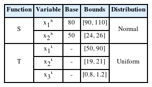
Case study: Design variables of nonlinear functions
Initial responses of each nonlinear function
3.2 Pre-training of Inverse Generator
The inverse generator was pre-trained using 20 sets of target data. In the first layer, the target responses were inputted. The size of the first layer was [590 × 1 × 1]. The middle layers define the core architecture of the network, where most of the computations and learning occur. There were five middle layers. The filter size was [20 × 1 × 1]. In the final layer, the output constituted the values for each target design variable. The final layer was [1 × 1 × 3]. The epoch was 10,000, and the batch size was 100% of the total training data. The learning rate was set to 0.001. The performance of the inverse generator was evaluated by the root mean square error (RMSE), which is the loss value of the actual and estimated design variables. The initial RMSE was 66.82, and the final RMSE was 0.4140. The elapsed time for pre-training was 3 min and 27 s. Because the final RMSE converged to near 0 compared with the initial RMSE, pre-training was performed properly. Therefore, an inverse generator that can output the estimated target design variables when the virtual target responses are inputted was constructed.
3.3 Training of DADDA
After pre-training the inverse generator, DADDA training was performed using 100 source responses. The first layer of the generator is defined to receive a random latent variable as input. The number of middle layers was 5, and it performed transposed convolution. The size of the filter was the same as that of the inverse generator. The final layer outputs the virtual target responses. The first layer of the discriminator receives the actual source responses and virtual target responses as inputs. The number of middle layers was 5, and it performed convolution. The size of the filter was the same as that of the inverse generator. The final layer was defined as the output score. The number of epochs was 1,000, and the batch size was 50% of the total training data. The generator and discriminator learning rates were 0.001, respectively. The performance of DADDA can be evaluated using the score when the loss of the GAN is optimal. If the score is 0.5, training is ideal. The initial score is 0.8165. After training was completed, the final score was 0.5045. Because the final score converged to approximately 0.5, training was performed properly. Consequently, DADDA generated virtual target responses and estimated the target design variables that affected the generated virtual target responses. The 100 generated virtual target responses are shown in Fig. 4. Each of the 100 virtual target responses was compared with the average of the 100 source responses to determine the accuracy of the virtual target responses. The weighted integrated factor (WIFac) is used as an accuracy index for time-series data [18]. WIFac is a single-valued index. It is calculated using an area comparison method rather than a point-to-point comparison between the two curves. Its value is between 0 and 1, and it can be expressed as
Comparison of actual source response and generated virtual target responses
where f [n] is the actual curve value, g[n] is the virtual curve value, and n is the variable of f and g. The similarity between f [n] and g[n] increases as WIFAC approaches 1.
The average accuracy of the 100 generated virtual target responses is shown in Table 2. When WIFac was multiplied by 100 and converted to an accuracy value, the average accuracy of the generated virtual target responses was 95.19%. The results for the estimated target design variables are presented in Fig. 5. The distribution of the estimated target design variables satisfied the initial target design variable bounds. Among the generated virtual target responses, the set of design variables with the highest accuracy was selected as the best set of target design variables. The best values were 52.81, 20.61, and 1.018 for
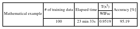
Case study: Average accuracy of generated target responses
Results of estimated target design variable distribution. (a) x1t. (b) x2t. (c) x3t
3.4 Validation of Design Solution
To validate the design solution, the estimated target design variables were reentered into the target nonlinear function. The validation accuracy calculated based on WIFac was 93.30%. Consequently, the performance of DADDA was validated using a mathematical example. The DADDA algorithm was coded with reference to the deep learning toolbox of MATLAB, version R2022a. The DADDA was trained on a 6-core i7-8700 CPU.
4 Application: Generative Design of Electric Vehicle
4.1 Simulation-based Data Acquisition
The source and target EVs were designed using Dymola [19], a 1D simulation tool, as shown in Fig. 6. Dymola is a modeling and simulation environment based on Modelica [20]. Information on the source and target design variables is presented in Table 3. There were three design variables (shock absorber damping, rubber bush stiffness, and anti-roll bar stiffness) in the source, and five design variables (shock absorber damping, rubber bush stiffness, anti-roll bar stiffness, battery position, and tire damping) in the target. One hundred pieces of values were randomly extracted from the distribution of each source design variable, and 20 pieces of values were randomly extracted from the distribution of each target design variable. The EVs were configured to enable autonomous driving in combination with a lane-keeping assist (LKA) system [21]. The driving around the elliptical track was simulated. The average driving speed was 30 km/h and the driving time was approximately 100 s. A total of 100 simulations were performed for the source and 20 simulations were performed for the target.
The source and target EVs design using Modelica/Dymola
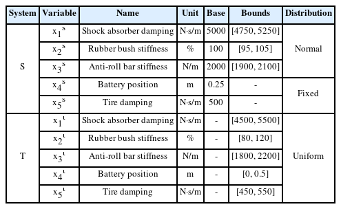
Application: Design variables of source and target EVs
The first dynamic response was the vibration acceleration in the vertical direction of the EVs and the second was the lateral deviation. The lateral deviation is the distance between the center point of the EVs and lane centerline. It was set not to exceed 0.2 m through the LKA. The vibration acceleration was acquired as image-type data and the lateral deviation was acquired as time-series data through simulation. The size of the image-type vibration acceleration data was [126 × 126 × 3] and the time series lateral deviation data was [1024 × 1 × 1]. To verify the simulation, a comparison with the experimental data of a motor-gear-bearing testbed similar to the EV drive system was performed. Because there is a limit on the entire EV system, a similar drive system was built through the testbed. The testbed and simulation model designed using Modelica are shown in Fig. 7. The vibration acceleration data for the two bearings were acquired according to the revolutions per minute (RPM) of the motor. The overall gear ratio was 7.75 : 1, and the vibration acceleration data were acquired when the RPM was increased from 300 to 1200. The vibration acceleration and fast Fourier transform (FFT) data for bearing 1 at 1200 RPM are shown in Fig. 8. To verify the accuracy of the simulation, the root mean square (RMS) of the vibration acceleration and the magnitude of the FFT were selected as comparison factors. The relative errors of the RMS and FFT magnitudes of the simulation for the testbed are listed in Table 4. The average RMS and FFT magnitude errors were 10.54% for RPM 300 and 4.75% for RPM 1200. Therefore, the Modelica-based simulation model was verified.
Qualitative illustration of the result of the missing marker reconstruction with a 40% missing ratio
Vibration acceleration and FFT data for bearing 1 at 1200 RPM. (a) Results of testbed. (b) Results of simulation
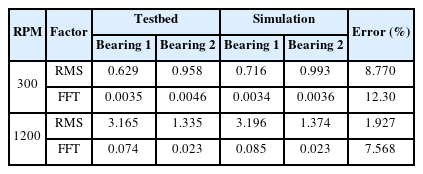
Relative errors of RMS and FFT magnitude of simulation for testbed
4.2 Pre-training of Inverse Generator Using Simulation-based Target Dynamic Responses
The target EV has multiple dynamic responses (i.e., vibration acceleration and lateral deviation); therefore, the inverse generator is configured as much as the number of each response. For each response, the inverse generator was pre-trained using 20 sets of target data. The size of the first layer for the image-type vibration acceleration data was [126 × 126 × 3], and the time series lateral deviation data was [1024 × 1 × 1]. There were five middle layers. The filter size for the image-type data was [6 × 6 × 1], and that for the time series data was [34 × 1 × 1]. The size of the final layer for both the responses was [1 × 1 × 5]. The epoch was 50,000, and the batch size was 100% of the total number of training data. The learning rate was set to 0.001. The initial RMSE was 15e6 and the final RMSE was 0.0284 for the image-type data. The initial RMSE was 15e6, and the final RMSE was 0.0258 for the time-series data. The elapsed time for pre-training the image-type data was 19 min 35 s, and the time series data was 17 min 51 s. Because each final RMSE converged to near 0 compared with the initial RMSEs, pre-training was performed properly.
4.3 Training of DADDA Using Simulation-based Source Dynamic Responses
The DADDA training was performed using source responses. To evaluate the performance of DADDA according to the amount of training data, 20, 40, 60, 80, and 100 source responses were selected as training data. The first layer of the generator was defined to receive a random latent variable as input. The number of middle layers was 5, and it performed transposed convolution. The size of the filter was the same as that of the inverse generator. The final layer outputs the virtual target responses. The first layer of the discriminator receives the actual source responses and virtual target responses as inputs. The number of middle layers was 5, and it was defined to perform convolution. The size of the filter was the same as that of the inverse generator. The number of epochs was 1000, and the batch size was 50% of the total training data. The generator and discriminator learning rates were 0.001, respectively. After the completion of training, the scores according to the number of training data were as follows: The initial and final scores were 0.876 and 0.513, respectively, when the number of training data was 20. The initial and final scores were 0.891 and 0.502, respectively, when the number of training data was 40. The initial and final scores were 0.813 and 0.496, respectively, when the number of training data was 60. The initial and final scores were 0.835 and 0.504, respectively, when the number of training data was 80. The initial and final scores were 0.839 and 0.507, respectively, when the number of training data was 100. Because the final scores converged to near 0.5, training was performed properly.
5 Results And Discussion
5.1 Generation of Virtual Target Responses
The 100 generated virtual target responses are shown in Fig. 9. Each of the 100 virtual target responses was compared with the average of the source responses according to the number of training data to determine the accuracy of the virtual target responses. WIFAC was used as an accuracy index for the time-series data. The structural similarity index measure (SSIM) was used as an accuracy index for image-type data [22]. SSIM calculates the distortion caused by the compression and transformation of an image by measuring the similarity between the generated and original image data. They have values between 0 and 1, and as the value approaches 1, the similarity between the two images increases. This can be expressed as
Results of generated virtual target responses
where μx is the average of image x; μy is the average of image y;

Application: Average accuracy of generated target responses according to the number of training data
5.2 Estimation of Target Design Variables
Among the generated virtual target responses, the set of design variables with the highest accuracy was selected as the best set of target design variables. The results of the estimated target design variables when the number of training data was 80 are shown in Fig. 10. The distribution of the estimated target design variables satisfied the design variable bounds. The design variable
Results of estimated target design variables
5.3 Validation of Design Solution
To validate the design solution, the estimated target design variables were entered into the Modelica-based target EV model. The validation accuracy according to the number of training data was as follows: It was 89.37% when the number of training data was 20, 89.44% when the number of training data was 40, 90.61% when the number of training data was 60, 90.44% when the number of data was 80, and 90.79% when the number of data was 100. In general, metamodel-based design optimization is a conventional design method. The metamodel was constructed using the design of the experiment, according to the design variable combinations. However, the type of response required to compose these metamodels must be a single value. In the case of time series or image-type data, it is difficult to apply to the existing metamodel; therefore, there is a limit to performing the conventional design method. In addition, to increase the reliability of the optimization results, a large number of experiments or simulations must be performed to verify the metamodel accuracy. Therefore, we propose and validate a new design method for EV using DADDA, a deep learning-based generative model.
6 Conclusions
Various technologies will continue to be combined in EVs. When a vehicle developer designs a new system, DADDA can satisfy the target performance in a short time using only a small amount of design information data. In this study, the training time required for the DADDA, including the inverse generator, to determine the target EV design solution was less than 1 h. The proposed design method was validated to determine the design solution of the target EV, which has a performance similar to that of the source EV by more than 90%, even when the number of design data for the target EV is small. The contributions of this study are as follows:
1) Existing data augmentation algorithms, such as GAN, generate virtual data using a small amount of actual data. However, from the viewpoint of predicting system responses, it is difficult to determine the design variables that affect the virtual responses generated by existing data augmentation algorithms. To solve this problem, the design variables affecting the virtual responses can be estimated by adding an inverse generator to GAN. Accordingly, the performance of a system can be predicted using only a small amount of design data, that is, without conducting a large number of experiments or simulations.
2) Through domain adaptation, virtual target responses that are similar to actual source responses can be generated. Therefore, a physically reasonable performance of an actual target system can be predicted. Consequently, a new system with a similar level of performance to that of an existing system can be designed using DADDA. These deep-learning-based approaches can be effectively applied during the front-loading design stage.
In future studies, we intend to proceed with a generative design with improved performance compared with the performance of the previously developed system. We plan to conduct a study to estimate optimal design variables that can improve the target performance by approximately 10–30% over the source performance.
Acknowledgement
This study was supported by the National Research Foundation of Korea (Grant No. 2022R1A2C2011034).
References
Biography
Yeongmin Yoo received Ph.D. in Mechanical Engineering at Yonsei University, Seoul, Korea in 2022. His research interests include multi-physics design optimization (MDO), prognostics and health management (PHM) and artificial intelligence & machine learning with applications to engineering systems.

Jongsoo Lee received B.S. and M.S. in Mechanical Engineering at Yonsei University, Seoul, Korea in 1988 and 1990, respectively and Ph.D. in Mechanical Engineering at Rensselaer Polytechnic Institute, Troy, NY in 1996. After a research associate at Rensselaer Rotorcraft Technology Center, he has been a professor of Mechanical Engineering at Yonsei University. His research adaptation interests include multi-physics design optimization (MDO), reliability-based robust engineering design, prognostics and health management (PHM) and industrial artificial intelligence.