Directed Graph-based Refinement of Three-dimensional Human Motion Data Using Spatial-temporal Information
Article information
Abstract
With recent advances in computer science, there is an increasing need to convert human motion to digital data for human body research. Skeleton motion data comprise human poses represented via joint angles or joint positions for each frame of captured motion. Three-dimensional (3D) skeleton motion data are widely used in various applications, such as virtual reality, robotics, and action recognition. However, they are often noisy and incomplete because of calibration errors, sensor noise, poor sensor resolution, and occlusion due to clothing. Data-driven models have been proposed to denoise and fill incomplete 3D skeleton motion data. However, they ignore the kinematic dependencies between joints and bones, which can act as noise in determining a marker position. Inspired by a directed graph neural network, we propose a novel model to fill and denoise the markers. This model can directly extract spatial information by creating bone data from joint data and temporal information from the long short-term memory layer. In addition, the proposed model can learn the connectivity between joints via an adaptive graph. On evaluation, the proposed model showed good refinement performance for unseen data with a different type of noise level and missing data in the learning process.
1 Introduction
With recent advances in computer science, there is an increasing need to convert human motion to digital data to research the behavior of the human body, such as gait analysis [1–3]. A motion capture system has been used to measure human or animal movement as sequential motion data [4]. Skeleton motion data generated using such a system comprise human poses represented via joint angles or positions for each frame [5]. Three-dimensional (3D) skeleton motion data are widely used in several applications, such as human-computer interactions [6], virtual reality [7], robotics [8–10], movie production [11], and action recognition [12–16].
Motion capture methods are broadly categorized into two: marker-based and markerless methods. Professional marker-based sensors, such as VICON [17] and Xsens [18], can capture motion data with high precision; however, they are expensive and only available in certain places. Markerless sensors, such as Microsoft Kinect can capture motion data at a low cost but the captured motion data have low precision and noise. The common issues with 3D skeleton motion data are that they are often noisy and incomplete due to calibration error, sensor noise, poor sensor resolution, and occlusion caused by clothing on body parts [19]. Fig. 1 shows types of incomplete data.
Illustration of types of incomplete data: (a) clean data, (b) data with 40% missing ratio, (c) data with 5-std Gaussian noise, and (d) coexisting data with 20% missing ratio and 3-std Gaussian noise
For effective data usage, data refinement should be performed beforehand [20–22]. Processing packages for refinement are provided in commercial motion capture systems, such as VICON [17], but they require manual user editing, which is labor- and time-intensive and results in unnatural movement because the kinematic information is not considered [11,20,21]. Therefore, several scholars have focused on motion data refinement.
The data refinement methods can be broadly categorized into nondate-driven and data-driven methods. Data-driven methods use a large amount of data to extract spatio-temporal patterns inherent in motion data. Notably, classical data-driven methods are action-specific; multiple actions could not be handled in a single model, and each action had to be trained separately [23,24]. Recently, deep learning methods—widely used data-driven methods—have succeeded in computer vision, image processing, pattern recognition, natural language processing, and computer graphics [25–28]. With advances in deep learning (DL) techniques, DL has also shown good results in the fields of motion data processing and generation [29–33]. Holden et al. [29,30] used a convolutional autoencoder model to encode human motion data into a low-dimensional manifold and proved that the model could decode them back into clean motion data. Although the model is nonaction-specific, the convolutional and pooling layers cause a jittery effect on the refined motion sequences [31]. Inspired by [29,30], Li [5] proposed an autoencoder model comprising a fully connected layer (FCL) and a bidirectional long short-term memory (LSTM) recurrent neural network (NN) [34,35] that can express sequence data better than a convolutional NN (CNN). The model imposes bone length loss and smooth loss in the learning process, thereby minimizing the jittery effect; it could generate data as a natural motion.
Notably, previous studies using FCL [5,19,36] and CNN [29,30] ignore the kinematic dependencies between joints and bones. Particularly, an FCL can act as noise in determining a missing marker’s position. For example, the shoulder joint is irrelevant in predicting the missing marker at the knee (Fig. 2(a)). It is more reasonable to predict the missing joint at the knee using the joints in the temporally surrounding frames and the spatially around the knee (Fig. 2(b)).
The process of updating a marker according to an FCL (a) and our desired result (b). The blue joints are used to update the orange node. The FCL can act as noise because it uses information from all unrelated joints to predict missing joints. Intuitively, the missing marker is significantly affected by the positions of the surrounding joints and bones. Such intuition makes a graph NN (GNN) that predicts missing markers using the surrounding joints and bones information (in the red curves) spatially and temporally. The green and yellow lines represent the spatial and temporal connectivities, respectively
In the field of human action recognition, many scholars have represented skeleton motion data as a graph with joints as nodes and bones as edges with prior knowledge of the local connection of human joints [14–16]. They have proven that bone information, which presents the direction and length of bones, is complementary to joint information and is a good modality for representing human motions. In addition, Lei [15] represented skeleton motion data as a directed acyclic graph and trained its connection adaptively. Inspired by [5] and [15], we propose a novel model that fills and denoises skeleton motion data using the information on relevant joints by representing the skeleton motion data as a directed acyclic graph. Particularly, we propose a novel graph autoencoder model that combines a directed graph network (DGN) block proposed in human action recognition [15] with a data refinement model [5] to refine incomplete 3D human motion data. The proposed model can not only directly use spatial information, which was included indirectly in previous studies by bone length loss, creating bone data from joint data, but can also handle the temporal information from the LSTM layer. Moreover, the proposed model can learn the dependency between joints from data via adaptive graph by putting joint and bone data into the network. The major contributions of this study are as follows.
1. To the best of our knowledge, this is the first time a directed acyclic GNN is applied to motion data refinement considering both spatial and temporal information. In addition, we demonstrate that it is highly effective in representing human motion data, even for refinement.
2. The proposed model is robust because it uses neighboring joints to predict missing joints, whereas other networks can be affected by irrelevant joints with severe noise or frequently missing joints.
3. The proposed model applies not only to various types of unseen data but also to input that has not been processed (e.g., rotation). Meanwhile, the previous models proceeded with data preprocessing for translation and rotation. There processes require the assumption that a particular joint must be measured, making it difficult to generalize many cases and time-consuming to preprocess. Because the proposed model considers the joint kinematic structure, it works well just by proceeding with data translation alone and can be generalized to various data.
4. On the CMU mocap dataset [37], the proposed model exceeded the state-of-the-art performance for 3D skeleton motion data refinement using three types of losses.
The code for our experiments is available on GitHub at https://github.com/cyun9601/BRA_DGN
2 Related Works
Incomplete data are due to the equipment noise and occlusion when measuring motion data. Thus, prior works eliminated noise from human data and predicted the positions of missing markers. The core of human data refinement is extracting and preserving the body’s intrinsic spatial-temporal pattern. As aforementioned, human data refinement methods can be broadly categorized into non-data-driven and data-driven methods.
2.1 Non-data-driven Methods
Classical data refinement methods use a linear time-invariant filter to remove noise. Brunderlin [38] proposed a multiresolution filter for motion data filtering in which the techniques used in the image and signal processing domain can also be applied to animated motion. Lee [39] proposed a computationally efficient smoothing technique to apply a filter mask to orientation data. However, these filter-based methods generate unnatural motion data because each joint is handled independently, which is the reason such methods could not use spatial information.
In subsequent studies, the linear dynamical system and Kalman filter theories were used to learn motion kinematic information. Shin [40] removed motion capture’s noise using Kalman filtering by mapping the performer’s movements to the animated character in real time. Li [41] proposed a DunaMMo model that comprised a Kalman filter and learns latent variables to fill missing data, whereas Lai [42] effectively reconstructed human data using the low-rank matrix completion theory and algorithm based on the relevance of the low-rank properties of representing human motion. In addition, Burke [43] refined missing markers by combining the Kalman filter and the low-rank matrix completion.
2.2 Data-driven Methods
Data-driven motion refinement methods have attracted considerable attention because the available amount of data has increased due to recent improvements in computer performance. Classical data-driven methods learn filter bases from motion data. For instance, Lou [23] proposed a model that learned a series of spatio-temporal filter bases from precaptured data to eliminate noise and outliers. Akhter [44] proposed a bilinear spatio-temporal basis that simultaneously exploits spatial and temporal regularity while maintaining generalization performance for new data, performing gap-filling, and denoising motion data.
Sparse representation has recently been widely used for denoising motion data. Xiao [45] assumed that incomplete poses could be represented as linear combinations of several poses and considered the missing marker problem in sparse representation. In addition, Xiao [24] eliminated motion data noise by partitioning the human body into five to gain a fine-grained pose representation. Xia [46] combined statistical and kinematic information and restored motion by imposing smoothness and bone length constraints. However, these methods were not generalized for any action type, requiring data to be learned for each action, and were not practically suitable for use.
With the recent rapid development of DL, DL is also widely used in motion data refinement. Holden [30] learned various human motion data using a convolutional autoencoder and interpolated them, whereas Mall [19] proposed a deep, bidirectional, recurrent framework to clean noisy and incomplete motion capture data. Li [5] proposed a bidirectional recurrent autoencoder (BRA) model and refined human motion data imposing kinematic constraints. In addition, Li [36] used a perceptual autoencoder to improve the bone length consistency and smoothness of refined motion data.
Previous studies indirectly extract kinematic information from human data by constraint. However, models that do not consider human structures do not maintain the kinematic information of human data. For example, an FCL uses the ankle joint, which does not significantly affect the shoulder joint prediction of the human body. In human action recognition—a representative research field using human data—many scholars have demonstrated that it is effective to represent human data in a directed graph for extracting bone information from human data. For example, Shi [15] classified various human behaviors by representing human data in an adaptive directed graph. Imbued by the aforementioned studies, we propose a model that can directly extract kinematic information from human data by representing them in an adaptive directed graph.
3 Method
Skeleton-based motion data comprise frame sequences, which are represented by 3D coordinates of joints. However, raw 3D skeleton motion data are often in-complete during the capturing process because of occlusion and noise, and they need to be refined before usage. To effectively refine incomplete data, we applied a DGN to a refinement model, resulting in robustness on rotation and deformation.
Fig. 3 illustrates a BRA with DGN block (BRA DGN) architecture proposed in this study. The architecture comprises the encoder that projects the input motion sequences to a hidden unit space and the decoder that projects it back to clean motion sequences. Each of the encoder and decoder contains a bidirectional LSTM to extract temporal information. This architecture, which changed an FCL in [15] to a DGN block, can extract spatial and temporal information by skeleton sequences into a graph structure.
The architecture of the proposed model: BRA DGN
We build bone data with joint data and represent the skeleton as an acyclic directed graph by expressing joints as nodes and bones as edges. Because we represent skeleton motion data as a directed graph, the DGN block can extract information using dependencies between joints and bones. A graph containing the attributes of nodes and edges enters several DGN blocks as input, resulting in graphs of the same structure as output. In each DGN block, the attributes of the nodes and edges are updated by their adjacent edges and nodes. The DGN blocks on the bottom layers extract the local information of nodes and edges while updating the attributes; the attributes of nodes and edges are aggregated and updated in a wider range on the top layers. Thus, as a graph enters the upper DGN block, it accumulates information from wider joints and nodes for refinement. Although this concept is similar to the principle of CNNs, the DGN block is designed for a directed acyclic graph. In this section, we describe the proposed model.
3.1 Notation
First, we describe the notations of skeleton motion data used in this article. Let M = [m1, m2, ..., mN] be a clean motion dataset with (N, C, T, V) shape, where N is the number of data, C is x, y, and z channel, T is the time sequence, and V is the number of joints. The mn = [p1, p2, ..., pT] that constitutes M is a sequence motion data with (C, T, V) shape, where pt = [x1, y1, z1, ..., xj, yj, zj] with (C, V) shape represents a pose data at a time in the temporal direction. We represent clean motion data as Y and missing data deformed from the clean motion data as X.
3.2 Bone Information
Studies of human action recognition [14–16] have proven that bone information is essential to represent human motion data. Bone information that represents the directions and lengths of bones is crucial because the position of each joint (bone) is determined by its connected bones (joints), and they are strongly coupled. In the motion refinement task, the bone length information is also crucial in that the length of the surrounding bone allows for accurate spatial prediction of missing markers. However, in previous studies [5,36,46,47], bone information has been indirectly used as a constraint in loss terms without extracting it from the data. Not limited to human action recognition, we used bone data to refine human motion by putting it in the proposed model’s input with the expectation of a better representation of the human skeleton because a better representation of the human skeleton yields better performance on the refinement of missing markers.
The bone information is defined by the difference between two connected joint coordinates. If two joint positions of v1 = (x1, y1, z1) and v2 = (x2, y2, z2) are given, where v2 is closer to the root joint than v1, the bone information of v1 and v2 is the difference between the two joint coordinates, i.e., ev1,v2 = (x1–x2, y1–y2, z1–z2).
3.3 Graph Construction
Li [5] and Holden [29,30] refined a motion sequence using CNN or FCL. Their methods ignored kinematic dependencies between joints and bones because there was no means to preserve or extract spatial information on their networks. We represent skeleton motion data as a directed acyclic graph by expressing joints as nodes and bones as edges (Fig. 4), similar to [15]. It is ideal to represent human motion data with a directed graph because the movement of each joint is physically controlled by adjacent joints, which are closer to the center. For example, the position of the wrist is determined by those of the shoulder and arm, which are closer to the root joint than that of the wrist. We set joint 12 as the root node and define the direction of bone to direct the joint farther from the center.
Illustration of the graph construction for CMU mocap dataset using 21 joints
In graph theory, an adjacency matrix represents the connection relationship between the nodes in an undirected graph. It is represented by 1 if the two nodes are connected and 0 otherwise. Although the matrix can indicate connectivity between nodes, it cannot indicate directions in an undirected graph. Therefore, to represent a human body as a directed graph, an incidence matrix is used to indicate the node directions. The directed graph in Fig. 5a is represented by an incidence matrix as follows:

Illustration of updating node and edge in a graph: (a) an original directed graph, (b) updating the green node using incoming orange edge and outgoing red edges. (c) updating the green edge using the orange source node and red target node
where A denotes the incidence matrix, and T denotes the transpose operation. Unlike the adjacent matrix, the rows and columns of the incidence matrix represent the indexes of the edges and nodes, respectively. The number “1” in the element of matrixes indicates the target node, which represents the incoming edges heading to a node, whereas the number “−1” in the element of matrixes indicates the source node, which denotes the outcoming edges emitting from a node. For example, the element at the second row and third column of the incidence matrix is 1 because e2 is heading to v3 and the element at the third row and second column of the incidence matrix is −1 because e3 is emitting from v2 (Fig. 5(a)).
To separate the source nodes from target nodes in the incidence matrix, we use A3 to denote the source nodes; it only contains the absolute value of the incidence matrix elements that are −1. Similarly, we use At to denote the target nodes; it only contains the absolute value of the incidence matrix elements that are 1. We set A3 and At as learnable parameters to form an adaptive body structure.
3.4 DGN Block
The DGN block is the main block of the proposed model, which is the basic block for a directed GNN [15]. This block extracts features by collecting information from connected peripheral nodes and edges in the spatial structure of the skeleton motion data. Because the BRA has limitations in extracting spatial information, we replaced the FCL with the DGN block. Figs. 5(b) and 5(c) shows how the nodes and edges are updated in the original graph by the DGN block. The DGN block performs two main processes: (1) aggregates the attributes and (2) updates the nodes and edges. The equations for aggregating and updating the input data are, respectively, as follows:
where Hv and He denotes the update functions of node and edge, respectively, and [·] denotes the stack operation of matrixes.
The incidence matrix is used to aggregate the nodes and edges based on their connected edges and nodes. In Equation (4), feAsT and feAtT denote the aggregations of the attributes contained in incoming edges and outgoing edges, respectively. The node update function, Hv, updates the attributes of a node by combining a particular node with incoming and outgoing edges and gives the output fv’. Similarly, in Equation (5), feAs and feAt denote the aggregations of attributes contained in the source and target nodes, respectively. The edge update function, He, updates the attributes of an edge by combining a particular edge with a source node and a target node and gives the output fe’.
4 Network Training
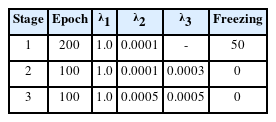
The proposed model is trained by minimizing three losses: position, bone length, and smooth losses. The total loss function is defined as
where λ1, λ2, and λ3 denote the weight coefficients of the three losses. Above all, it is crucial to minimize the position loss because it ensures the refined motion sequence has a smaller Euclidean distance from the clean motion sequence than the other losses do for generating natural motion. Hence, the proposed model is trained in three stages via changing the weight coefficients. Table 1 describes the parameters used in each stage. The parameters of the incidence matrix are fixed until other parameters are learned to some extent at the first stage to maintain prior knowledge of the human body’s kinematic structure. The batch size is set to be 16, and Adam [48], an adaptive gradient descent algorithm, is used to optimize the parameters.
Hyperparameter table
4.1 Loss Function
4.1.1 Position Loss
The most commonly used loss function for data refinement is L2 loss between the network output and ground truth. We define this loss as position loss, which is the most critical loss regarding the distance between the predicted and actual joint positions. Fig. 6a shows the predicted and actual joint positions when the predicted position is inaccurate. Position loss is formulated as follows, where ||·||2 denotes the L2 norm.
Types of error between a predicted and clean position of the markers: (a) position error, (b) bone length error, and (c) smooth error. The black and green dots represent the label and predicted joints, respectively. The red lines in (a) represent the distance error, and the red circles in (b) and (c) represent the points at the same L2 distance from the label position
According to the results of the previous studies that used only position loss, the output motion sequence remains jittery [29,30]. Meanwhile, in [5,30,36], which are the most closely related studies to this study, the bone length and smooth losses were used to remove the jittery effect.
4.1.2 Bone Length Loss
Bone length constraints have been used in many studies [5,36,46] to extract kinematic and statistical characteristics by putting prior knowledge of bone length into the model. In Fig. 6(b), although the two predicted results (green dots) differ in the prediction of joint position, the position losses of both results are the same because the distances between the label (in the red circle) and both results are the same. For the natural motion sequences, the bone length loss is needed to keep the bone length constant. The bone length loss is defined as
where Lb denotes the bone length of clean data, and lb denotes the predicted value of the joint coordinates between the two ends of the bone, calculated with the L2 norm.
4.1.3 Smooth Loss
The joint can be jittery in the temporal direction, whereas the position and bone length losses are the same (Fig. 6(c)). Because the motion of the human body should be smooth in the temporal direction, non-data-driven methods impose smoothness to refine the natural motion sequences by enforcing C2 continuity on each feature dimension via a smoothness penalty term [49–51]. Recently, Li [5,36] added a smoothness constraint at the training phase to train a DL model. Let O be a symmetric tridiagonal matrix, defined by
Then, the smooth loss is defined by
where X’, represented by (T+2)×(C×V), is derived from X by repeating the border elements, i.e., p0 = p1 and pT = pT+1.
5 Experiment and Results
5.1 Generating Incomplete Data
We use the CMU Motion Capture Database [37]. With 31 markers attached to actors, the motion data were captured with an optical motion capture system. These data were converted from the joint angle representation in the original dataset to the 3D joint position, subsampled to 60 frames per second, and separated into overlapping windows of 64 frames (overlapped by 32 frames). Only 21 of the most relevant joints were preserved (Fig. 4). The proposed model applies to not only data from 64 frames but also data from other various frames.
Notably, the location and direction of skeleton motion data in the human motion data can change with the time they are captured. Similar to previous studies [5,30], not only the global translation is removed by subtracting the root joint position from the original data but also the global rotation around the Y-axis is removed. Finally, we subtracted the mean pose from the original data and divided the absolute maximum value in each coordinate direction to normalize the data into [−1, 1]. This preprocessing process helps a particular joint to exist in stochastically similar locations, making it easier for the model to predict.
The purpose of this study is to generate clean data from corrupted data with occlusion or noise. Because CMU mocap data are clean data, we have to create corrupted data by making missing markers or adding noise to train the model. As human data are measured with a single measuring device, the types of noises within an entire data can be considered the same. Therefore, we created and then added the same type of white noise to the position values of all joints.
5.2 Comparisons with Baselines
In this section, we compare the performances of the proposed model (BRA DGN), CNN [29,30], BRA [5], two encoder-bidirectional-decoder (EBD), and EBD DGN. Although the last two models have the same architecture as BRA and BRA DGN, they do not impose smoothness and bone length constraints during the training phase. We compared these models with the following three experiments to evaluate the performance of the proposed model. All experiments were conducted on a workstation equipped with an Intel Core i9-10900X CPU and RTX 3090.
Missing marker reconstruction. It is about how well a model can predict a missing marker without noise. This experiment demonstrates the reconstruction performance of the model—this case borders on marker-based with little noise.
Missing marker reconstruction with noise. We evaluate the refinement performance on data with noise and missing markers coexisting together. It is close to a markerless setup where noise and missing occur a lot.
Missing marker reconstruction without standardizing. Standardizing skeleton motion data is intended to improve the model’s predictive performance by helping the joint stay within a certain range. However, because the DGN block predicts missing markers using the positions of the surrounding joints, it will predict missing markers well without standardizing. Therefore, we evaluate the reconstruction performance without standardizing.
In all three experiments, the model’s performance was evaluated by position, bone length, and smooth errors. The position error is the most critical because we aim to refine incomplete data. If the position error is reduced, the bone length error is reduced too; the smooth error is also present in the clean data because it represents the difference in the positions of the joints between neighboring frames, and it is desirable for the smooth loss of the refined data to have a similar value with that of the clean data. Hence, we represented the smooth error by the difference between the smooth losses of the clean and refined data. For cross-validation, we randomly used 70% of the CMU mocap data for training and the remainder for testing. The results of the first experiment are shown in Fig. 7 as an example.
Qualitative illustration of the result of the missing marker reconstruction with a 40% missing ratio
We can qualitatively evaluate the model’s performance from Fig. 7. Compared with other models, our proposed model (BRA DGN), showed the best performance in terms of the position and bone length losses. Although other models’ predicted node positions and, especially, bone lengths show a big difference from those of the label, BRA DGN produced a prediction almost similar to the label. Such an outstanding result of BRA DGN was possible because it not only reflects each loss but also considers the kinematic dependency of human structure using the directed graph.
5.2.1 Missing Marker Reconstruction
We need to evaluate the model’s performance when the missing types of the training and test data differ because we do not know how much of the actual measured data has been occluded. Therefore, we trained 40% random missing data without noise to evaluate the refinement performance of the model on missing data. Then, we tested the model on randomly missing data or data with few joints missing from the entire frame.
EBD DGN and BRA DGN showed the best performance in position and bone length errors, respectively (Fig. 8 and Table 2). Hence, models representing 3D human structures as graphs effectively extract spatial information from data, and the data generated via these models show high visual quality (Fig. 7). Moreover, the graph-based models generate the refined data with a similar smooth loss to that of the clean data. For the last two rows in Fig. 8 where the particular nodes are missing from all frames, other models that extract only temporal information; however, have to be refined with spatial information only, resulting in significant performance degradation.
Performance comparison of models trained with 40% randomly missing data
Comparison of qualitative experimental results on 40% randomly missing data
5.2.2 Missing Marker Reconstruction with Noise
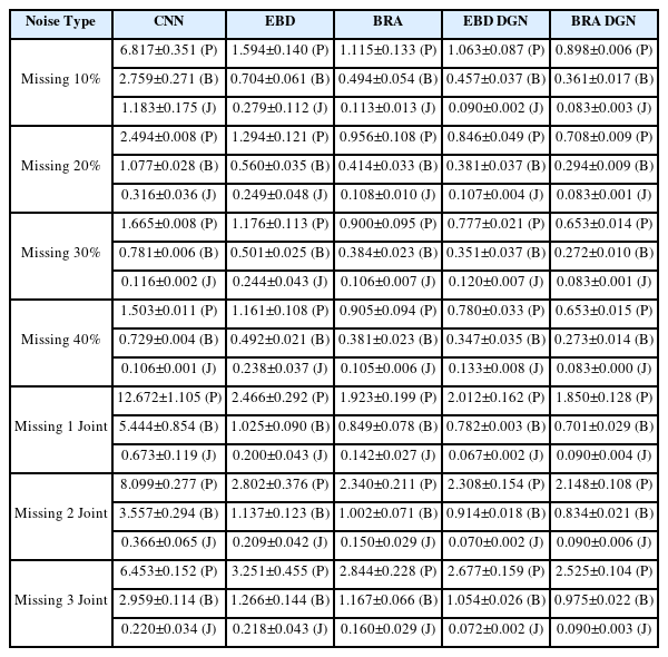
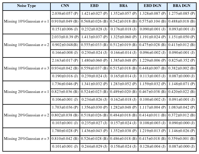
In this subsection, we compare the refinement performance of models on data with both occlusion and noise. For the comparison, we train the models with 20% missing and 3-std noise data and test them with various types of incomplete data. The results are described in Fig. 9 and Table 3. BRA DGN and EBD DGN showed the best performance in the position and bone length errors, respectively. Although the test data differed significantly from the training data, they showed almost the same performance as before. However, BRA showed severe performance degradation as the difference between the training and test data increased, attributable to the failure of the FCL to extract the spatial information of the human body.

Performance comparison of models trained with 20% randomly missing data with 3-std Gaussian noise
Comparison of qualitative experimental results on 20% randomly missing data with 3-std Gaussian noise
5.2.3 Missing Marker Reconstruction without Standardizing
The preprocessing process is intended to help the model learn by making markers in a stochastically specific position. In Subsection 5.1, global rotation was removed to preprocess the 3D human data, which has a limitation that several joints must be measured to make the skeleton motion data look in a particular direction. However, if the model considers the spatial information based on GNN, it is possible to predict the missing joints without the aid of this preprocessing.
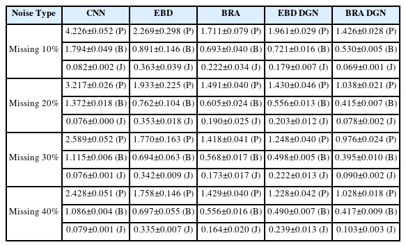
We trained the model with 40% missing ratio data without noise and then tested on various missing ratio data (Fig. 10 and Table 4). Notably, the data used in this case was not rotated. The proposed model was unaffected by rotation, but other models were significantly affected because they failed to consider spatial information. Hence, the proposed model has the advantage of having fewer joints that must be measured to rotate not only the skeleton motion data but also any other data and reduce the time required to standardize the data.
Performance comparison of models trained with 40% randomly missing data without standardization
Comparison of qualitative experimental results on 40% randomly missing data without standardization
5.3 Hyperparameters for Comparative Models
Finally, we experimented with varying the number of DGN blocks to find the optimal count by observing the training time and error across three types of loss. The training was conducted with 10% random missing data without Gaussian noise. The results, including the number of parameters for each model, training time, and each error are presented in Table 5. The total loss reached its minimum with the use of three DGN Blocks, with both position loss and smooth loss registering their lowest values at this configuration. However, performance started to decline when the number of DGN Blocks exceeded three, attributable to a rise in the number of parameters, which in turn led to overfitting on the training dataset.
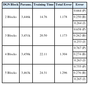
Comparisons for number of DGN blocks for BRA DGN
In addition, we ensured a fair experimental setting by comparing the parameters of each comparative model. The parameters for each model are outlined in Table 6. While CNN exhibits fewer parameters compared to other models, the remaining four models have nearly identical model parameters. Notably, the proposed BRA DGN model demonstrates superior performance despite having fewer parameters than the other models. This provides clear and indisputable evidence of the effectiveness of the proposed model.
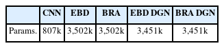
Model parameters for each comparative model
6 Conclusion
Refining 3D skeleton motion data is an indispensable step in preprocessing motion data, particularly for inexpensive noisy motion capture devices. We propose a graph-based model that considers spatio-temporal information for refining 3D human data. An autoencoder comprising FCLs has been used in previous studies for human data refinement, but the positions of all joints are considered to predict that of missing markers. However, the incomplete joint is only affected by the neighboring joints in the human structure, whereas the distant joints are irrelevant for refinement. To preserve the kinematic dependency of the human structure, we represent the human structure as a graph by expressing joints as nodes and bones as edges. Because the joints far from the center are affected by the joint near to the center, we used an adaptive directed GNN to extract the spatial information. In addition, we used an LSTM layer for the hidden units projected from the encoder to extract temporary information. To verify the superiority of the proposed model, we trained and tested the model in three manners: missing marker reconstruction, missing marker reconstruction with noise, and missing marker reconstruction without standardizing. Comparing the refinement performance of our model with those of others, that of our model was the best, and our model effectively extracted the spatial information of the human body.
Acknowledgement(s)
This research was financially supported by the Institute of Civil Military Technology Cooperation funded by the Defense Acquisition Program Administration and Ministry of Trade, Industry and Energy of Korean government under grant No. 19-CM-GU-01.
Notes
Conflict of interest
The authors declare no competing interests.
References
Biography

Changyun Choi received the M.S. degree in Mechanical Engineering from Pohang University of Science and Technology (POSTECH), Republic of Korea, in 2021. He has been a Data Scientist with Minds and Company, Republic of Korea, since 2019. His research interests include the application of artificial intelligence in assembly sequence planning in the automobile industry, reinforcement learning, autonomous car, and digital signal processing.
Jongmok Lee received the B.S. degree from Pohang University of Science and Technology (POSTECH), Republic of Korea, in 2021. He is currently pursuing the M.S./Ph.D. degree with the Industrial Artificial Intelligence Laboratory, POSTECH, Republic of Korea. His research interests include artificial intelligence (AI) with physics-informed neural networks and graph neural networks.

Hyun-Joon Chung received M.S. and Ph.D degrees in mechanical engineering from the University of Lowa City, USA, in 2005 and 2009, respectively. He was a Research Assistant and Postdoctoral Research Scholar in the Center for Computer Aided Design, from 2005 to 2015. He joined the Korea Institute of Robotics and Technology Convergence as a Senior Researcher in 2015. He is currently a Principal Researcher and the Head of AI Robotics Center in Korea Institute of Robotics and Technology Convergence. He serves as a General Affairs Director of Field Robot Society in Korea. His research interests include dynamics and control, optimization algorithms, computational decision making, modeling and simulation, and robotics.

Jaejung Park received the B.S. degree from Pohang University of Science and Technology (POSTECH), Republic of Korea, in 2021. He is currently pursuing the M.S./Ph.D. degree with the Industrial Artificial Intelligence Laboratory, POSTECH, Republic of Korea. His research interests include the application of artificial intelligence (AI) in material science and mechanical systems.

Bumsoo Park received his B.S. and M.S in Mechanical Engineering from the Ulsan National Institute of Science and Technology (UNIST), and Ph.D. in Mechanical Engineering from the Rensselaer Polytechnic Institute (RPI), Troy, NY, USA. He is currently a post-doctoral researcher at the Korea Advanced Institute of Science and Technology (KAIST). His research interests include the development of learning control algorithms for mechanical systems with complex dynamics, and deep learning applications to mechanical systems.
Seokman Sohn received his B.S. in Mechanical Engineering from Yonsei University in 1993. He then received his M.S. degree from Korea Advanced Institute of Science and Technology in 1995. He had researched the diagnosis of rotating machinery. He is currently a leader in worker safety technology team of Korea Electric Power Research Institute at KEPCO. His major research field is the worker safety technology development.

Seungchul Lee received the B.S. degree in Mechanical and Aerospace Engineering from Seoul National University, Seoul, Republic of Korea; the M.S. and Ph.D. degrees in Mechanical Engineering from the University of Michigan, Ann Arbor, MI, USA, in 2008 and 2010, respectively. He has been an Associate Professor with the Department of Mechanical Engineering, Korea Advanced Institute of Science and Technology, since 2023. His research focuses on industrial artificial intelligence for mechanical systems, smart manufacturing, materials, and healthcare. He extends his research work to both knowledge-guided AI and AI-driven knowledge discovery.