

 E-mail
 Print
Print facebook
 twitter
 Linkedin
 google+
1. Introduction
Machines emit sounds which include operational and process information as they work. In the metal cutting industry, operators next to the machine constantly listen to the operational sound. They easily distinguish operational information such as axis movements, spindle running, and cutting engagement. A well-experienced operator is even able to identify subtle changes in the operational sound caused by the fault of the machine or cutting failure, which indicates sounds from machines contain ample information about the operation. Sound has been receiving attentions for monitoring machines.
Acoustic emission and vibration have been frequently used to monitor manufacturing processes [1,2]. The measuring frequency range is from 25 kHz to 400 kHz, which is beneficial to monitor the details such as cracks in materials or plastic deformation. However, it is not a practical area for monitoring general manufacturing processes such as cutting with low tool rotations and handling materials. Conditioning devices are also required to amplify the sensor signal, which is not also suitable for IoT solutions requiring reduced costs and lower footprints. Vibration sensors are also widely used for monitoring processes. The measurement range is from 5 Hz to 10 kHz, and it is mainly used to monitor rotary machines consisting of motors, shafts, and bearings [3]. However, it also requires data acquisition devices to cover the frequency range.
Microphones are a candidate for IoT applications in manufacturing. They are commonly used as measuring sounds at audible frequency range typically from 20 Hz to 20 kHz without additional conditioning devices. In recent manufacturing applications, a single microphone was used to monitor milling tool wear [4] and the status of carbon-fiber-reinforced polymer (CFRP) milling operations [5]. However, it is vulnerable to external noise, which can be reduced by the localization from multiple microphones or sensor fusion techniques. A bundle of microphones was used to estimate milling conditions [6] while further noise reduction methods were not presented. Filtering using multi-resolution techniques [7] would reduce the noise after signal acquisition.
Our group has developed a stethoscope-based internal sound sensor. It consists of a stethoscope and a USB microphone attached to a rubber hose to record internal sound. The details of sensor structure and system identification were presented in [8]. It was applied to detect collision of an industrial robot [8] and anomaly when the robot holds too heavy weight [9]. In addition, the sensor was used to predict the running state of the components of CNC machines via convolutional neural network (CNN) [10]. Recently, we have presented an application to estimate the running state of generators in a powerhouse [11]. Especially, the Mel spectrum feature extraction technique was used to convert sound signal and the converted two-dimensional (2D) image for the input of CNN. The CNN modelŌĆÖs output is the probability of generatorsŌĆÖ running state. As a result, the accuracy of prediction is 95%, showing potentials for non-invasive and affordable estimation of the operational state of machines.
As monitoring machine operational state is regarded as more and more crucial with autonomous operations and the expanded flexible manufacturing systems, this study extends our previous works. Although programmable logic controllers (PLCs) or computer numerical controllers (CNCs) with sensors can count the produced parts, the resources for installing additional hardware and downtime are unavoidable on existing manufacturing systems. Using the developed internal sound sensor, the cutting state prediction function was successfully implemented while there were no interruptions of ongoing production. It was also possible to block noises from other machines without any filtering processes.
In recent manufacturing process monitoring, sound signals have been converted to features, and used for the input of training data for deep neural network (DNN). In feature extraction step, various multi-resolution signal analysis techniques have been proposed: short-time Fourier transform (STFT) [8,9], wavelet transform (WT) [4,7,12,13], Mel-spectrum feature extraction [11], and Hilbert-Huang transform (HHT) [14]. These techniques convert time-domain one-dimensional (1D) sound signals to time-frequency 2D information and extract features in a certain frequency range. The methods have been vastly used for different applications and studies.
After the feature extraction step, the outputs are used as input data for training and testing machine learning models. Machine learning techniques like K-mean clustering [15], support vector machine (SVM) [16,17], and principal component analysis (PCA) [18] have been used after fast Fourier transform (FFT). In addition, 2D spectrograms were mostly utilized as input of DNN. STFT spectrogram was used to train CNN [8,19,20] and autoencoder [9], and Log-Mel spectrogram [21] was used in similar ways.
Recent studies have focused on advanced and lightweight methods of sound analysis for IoT solutions. Group method of data handling (GMDH) was used as a self-organizing neural network (NN) for monitoring machining with sound for higher performance than back-propagation based NN [7]. In another study, features are extracted as parameters, then used for two layers of kernel extreme learning machines (KELMs) [22]. KELM is a simple DNN consisting of a single hidden layer of kernel functions for fast speed and less training data. Another study introduced XNOR-net [23], a bit-wise operation of CNN to simplify audio classification for use in edge devices. Furthermore, the accumulation of real-time serial-to-parallel converter (ARS) was proposed, which is the accumulation of low frequency area of machine sound, showing precise machine state prediction with less computation than STFT and WT [12].
Acoustic signals have been mostly used for monitoring machine conditions. For predictive maintenance and prognostic health monitoring, fault diagnosis of rotary components is studied. The related studies of fault diagnosis systems using audio and vibration signals were reviewed in [24], and DNN was utilized in the latest study. Another study area using sounds is tool condition monitoring (TCM) estimating tool wear to monitor product quality and plan tool change. Recent studies are trying to utilize machine learning [16,22]. In another research area, estimating machining parameters from sound was reported in a few studies. The method was also applied to turning processes [25]. As regression methods, [18] estimated CNC parameters such as depth of cut, width of cut, federate, and spindle speed from support vector regression (SVR) and neural network-based regression (NNR). Especially, recent studies have focused on finding anomalies in manufacturing processes. In [26,27], anomaly from a surface mounted device machine was found from recurrent neural network (RNN) and autoencoder. In the study, STFT and Mel-frequency cepstral coefficients (MFCC) of acoustic signal were used as input data. The autoencoder was also utilized to detect when an industrial robot is lifting heavier weight than usual state [9]. Similarly, [18] used the combination of sound and vibration to estimate anomaly of a fabric cutting machine: loose knife, no knife, and no belt. In another study bottle damage from filling process was detected by sound [14]. Studies of finding anomalies from acoustic signals have been recently reviewed [28], showing that anomaly detection from acoustic signals is an emerging area of fault diagnosis.
From the reviewed methods and applications, this study presents a new application of sound sensing for real-time monitoring cutting time and productivity of a tube cutting machine without any interruptions of production on a real shop floor. To compare performances according to sensor types and places, three sound sensors were used: an external microphone on top of the machine enclosure and two internal sound sensors on top of the machine enclosure and the machine base. The 2D Log-Mel spectrum was used as the feature of the sound. As is analogous to an operator who can figure out the operational information by listening to the sound, the Mel scale was employed, which mimics human hearing, for converting sound signals into 2D time-frequency information. With the Log-Mel spectrum features, 2D CNN was adopted for the training model to predict cutting state sound pattern matching. Unknown and untrained data were utilized for the evaluation of the trained CNN model to predict the cutting state. As the input feature variable, the effects of the size of the time frame of sound signals were analyzed. It also presents a method to extract productivity information as part counting function from the results of cutting state prediction, which is a contribution of this paper. Moreover, the method was successfully implemented in real production monitoring and the performance of monitoring response time was also evaluated.
2. Target Machine and Sensor Deployment
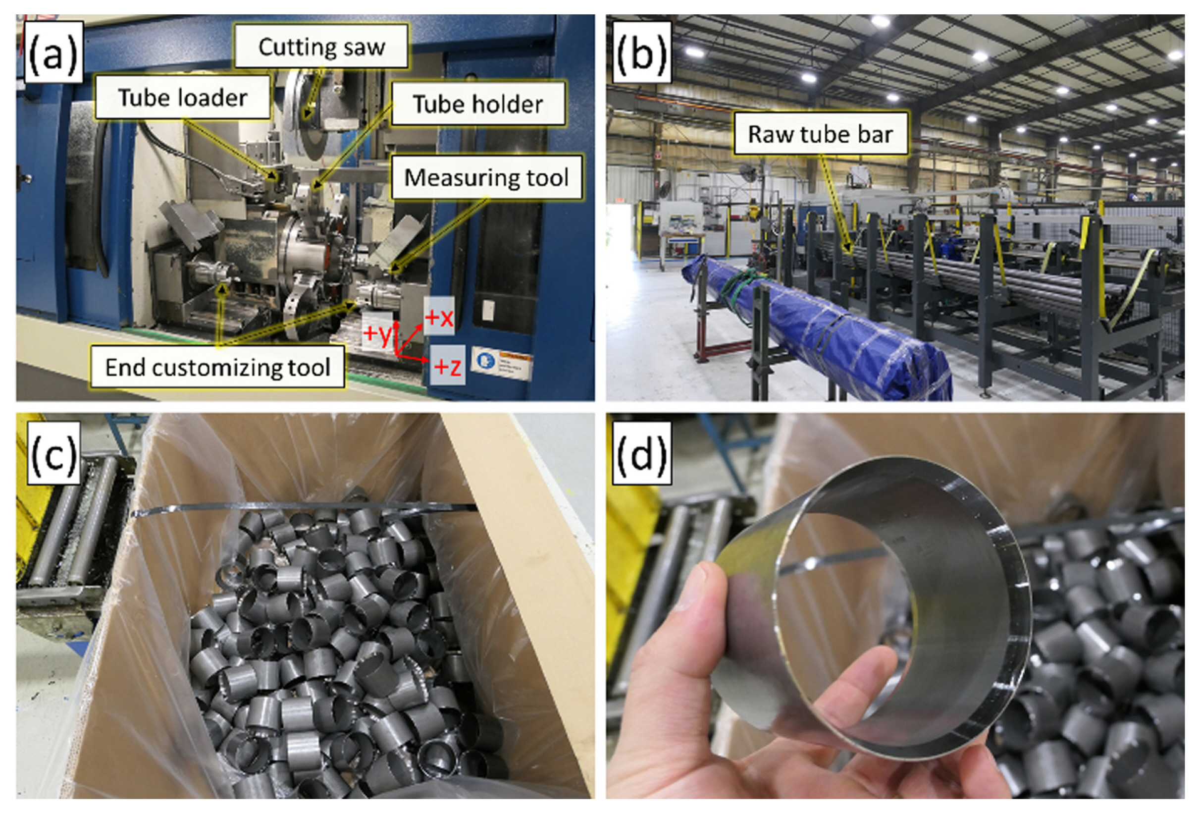
The target machine is a horizontal tube cutting CNC machine on a real shop floor. There are tens of other manufacturing machines close to the machine and in the same area, which results in a loud and noisy environment. The tube cutting machine cuts approximately a 6-meter-long metal tube bar into tens of tubing parts. The configuration in the working area and the manufactured parts of the machine are shown in Fig. 1. The main components inside the working area ((a)) the tube loader, the cutting saw, the tube holder, and the end-customizing and chamfering tool. The tube bar feeding area picture is shown in Fig. 1(b). The manufactured parts and the closeup picture of a sample part are shown in Fig. 1(c) and 1(d), respectively. Table 1 shows the manufacturing steps of the tubing part.
The rotating step, which is the tube holder rotates at 90┬░ in the positive z-direction (Fig. 1(a)), is conducted between steps 3-1 (Cutting), 3-2 (End customizing), 3-3 (Measuring), and 4 (Discharging). Steps 3-1 (Cutting), 3-2 (End customizing), and 3-3 (Measuring) are performed simultaneously. In addition, step 1 (Loading) and step 4 (Discharging) are performed at the same time. The steps are repeated in every part of the production. Step 3-1 (Bar cutting) is always performed in every operation, although steps 3-2 (End customizing) and 3-3 (Measuring) are optional. Moreover, the material of the tube bars and the cutting parameters such as spindle speed, feed rate, and so on can be differed by the part design and the operation. More importantly, the cutting time per part varies approximately from 2 to 4 seconds depending on the material and part design.
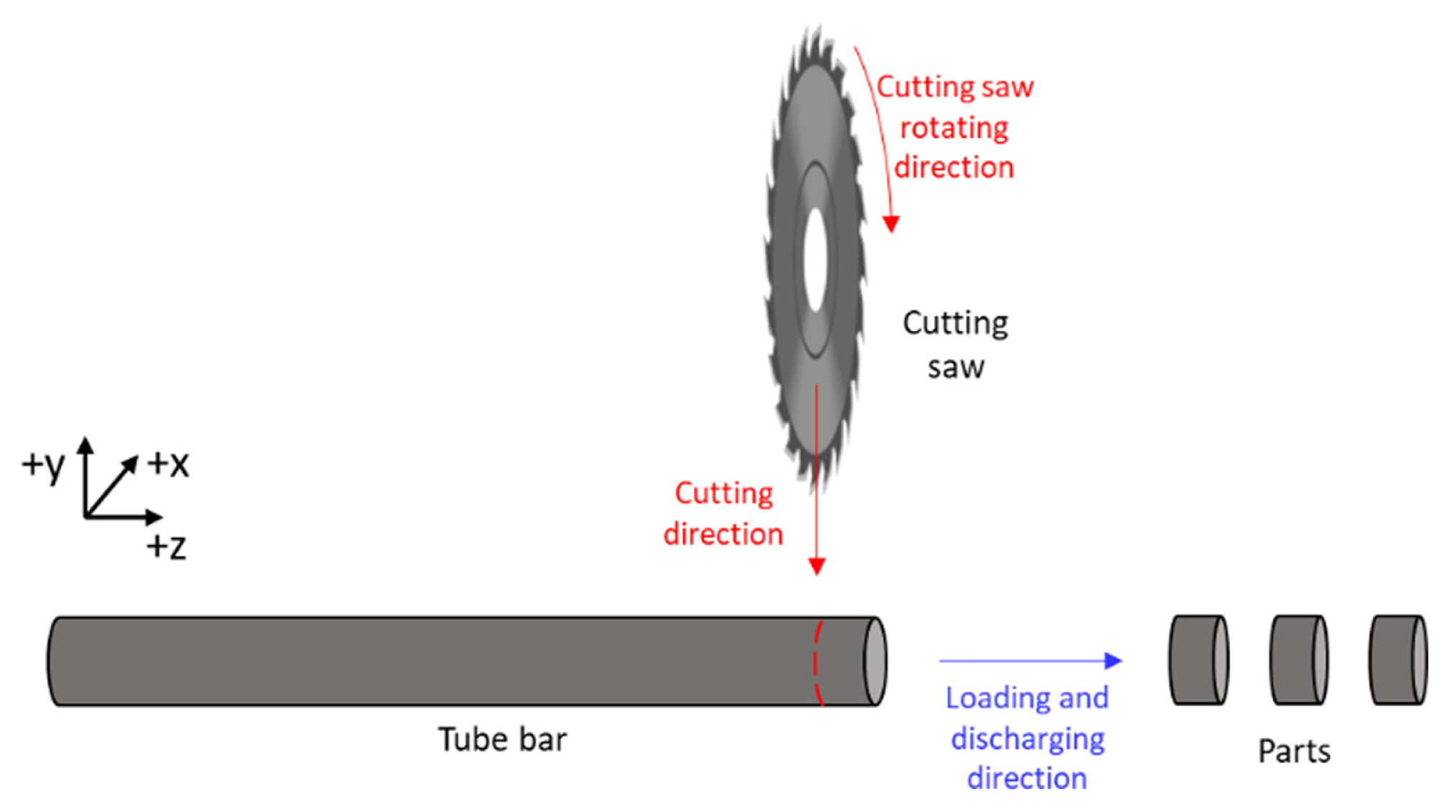
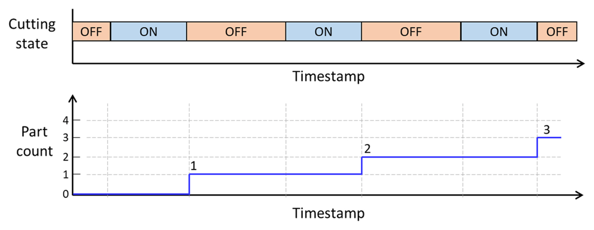
The simplified tube cutting manufacturing diagram is shown in Fig. 2. The number of bar cuttings results in the number of parts. In other words, the cutting count represents the part count as Fig. 3. When the cutting ends, the part count increases by one. The condition of the cutting saw mostly affects the quality of the part. In this factory, practically, the cutting saw is replaced when the actual cutting time is near the guaranteed cutting time suggested by the cutting saw manufacturer. They rely on the manually written operation logs for the cutting saw usage to determine the cutting saw replacement. Therefore, knowing the exact accumulated used time of the cutting saw is the most important to control the effectiveness of the cutting operation.
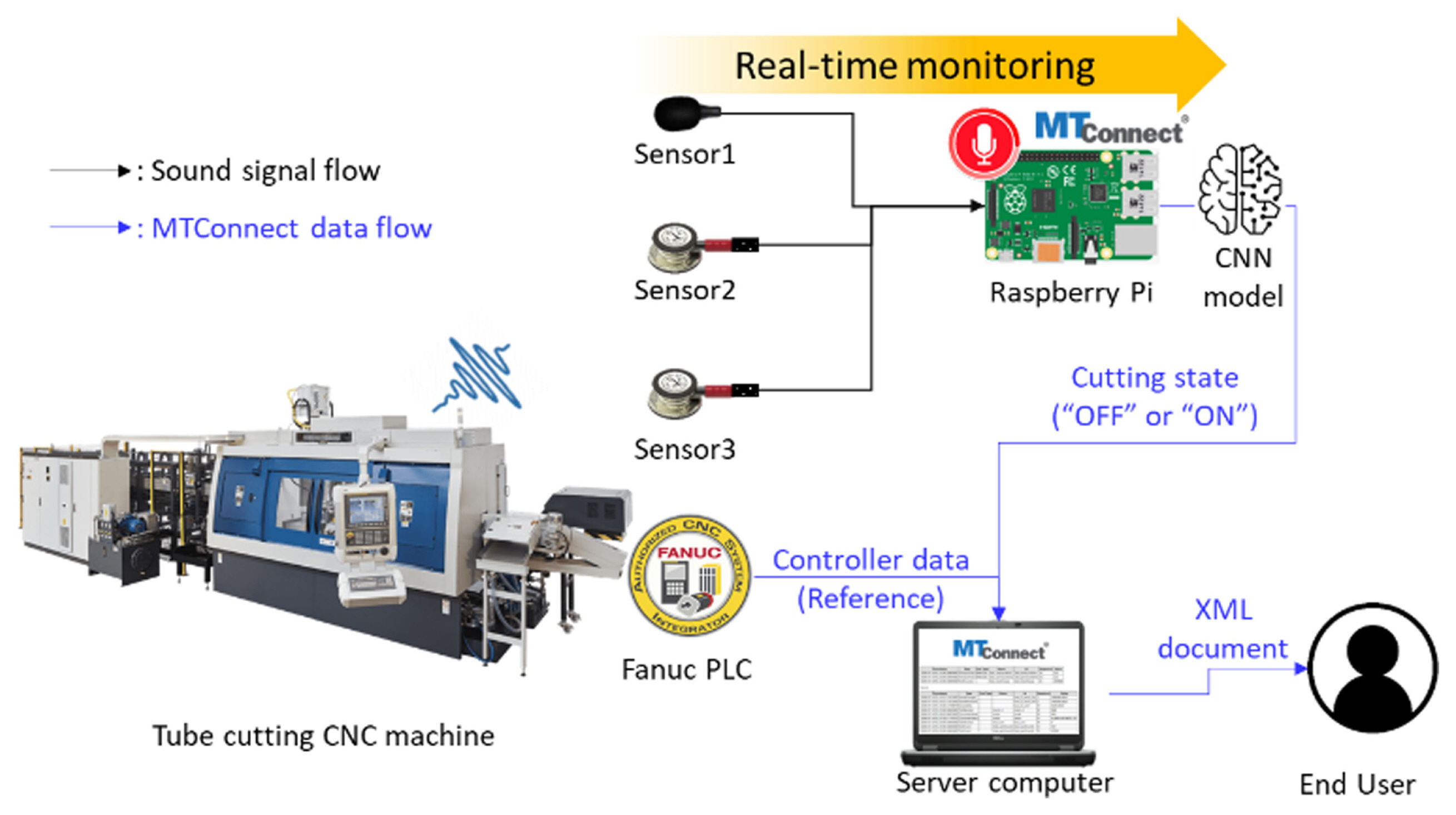
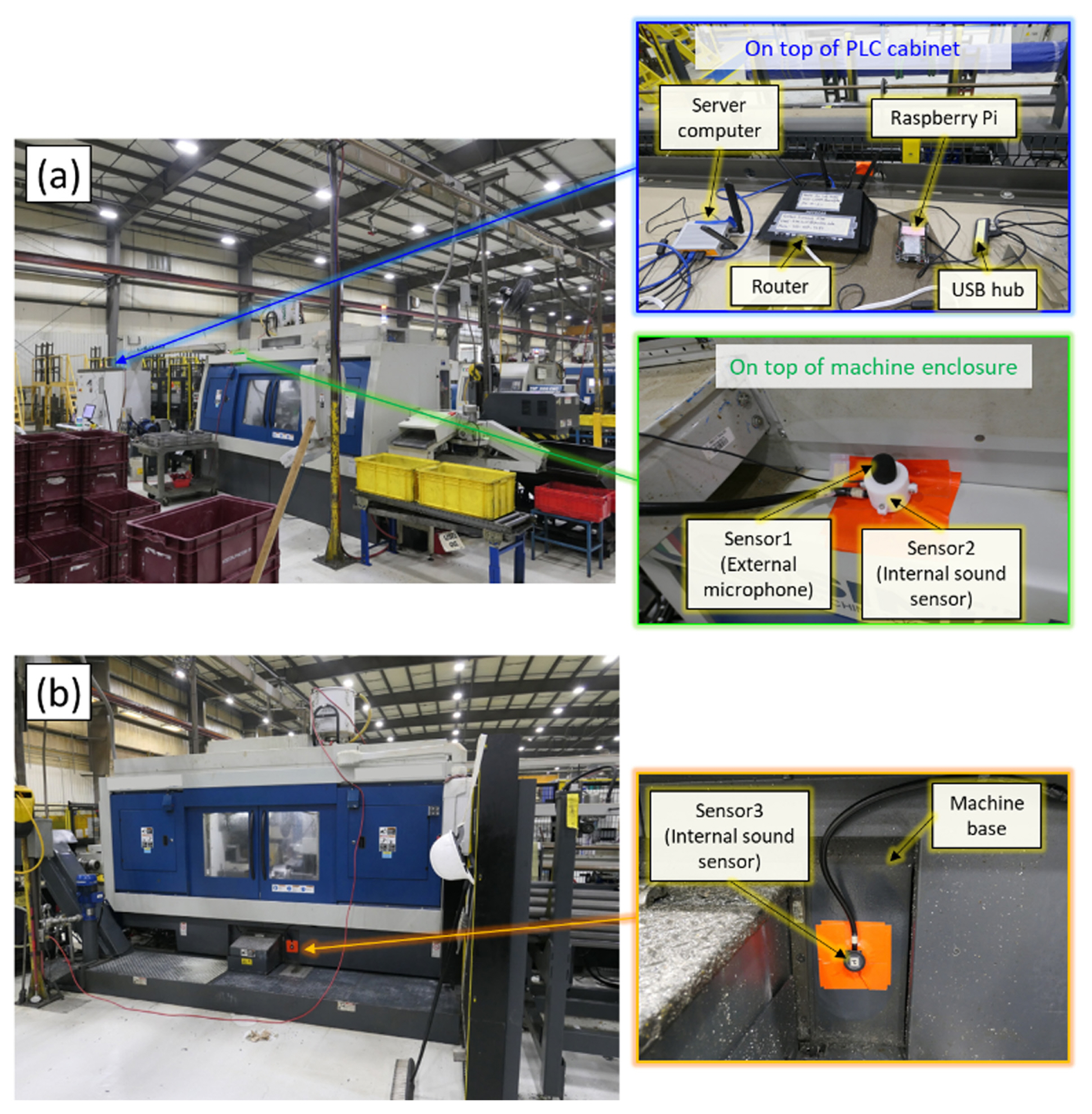
The overview of the sound monitoring system is illustrated in Fig. 4. To monitor sound from the tube cutting machine, the MTConnect framework was used as a data-to-information protocol. Three sound sensors were attached to the machine and connected to an edge computer (Raspberry Pi 4 B, Raspberry Pi®). The edge computer collects sound signals from each sensor as well as runs the MTConnect adapter which indicates the cutting state based on sound signals. To verify the productivity performance of the cutting state prediction model, which is further described in the following sections, an MTConnect adapter application written by C# using Fanuc® FOCAS2 library was developed to collect NC data. An industrial compact server computer (CL210, OnLogic®) aggregates in the MTConnect agent not only NC data from the machine but also the cutting state from the edge computer so that end users are able to know the cutting state of the machine as an XML document format remotely in real-time.
Hardware and sensor deployments are shown in Fig. 5. One external microphone (K053, FIFINE®), denoted by sensor 1 (Fig. 5(a)), was deployed on top of the envelope of the machine to capture airborne sound from the machine. To capture the internal sound from the target surface, the internal sound sensor which consists of a stethoscope (Littmann Classic III, 3M®) and the same USB microphone as sensor 1. The USB microphone was inserted into to the end of the hose of the stethoscope. Two internal sound sensors, denoted by sensor 2 (Fig. 5(a)) and sensor 3 (Fig. 5(b)), were deployed on the same placement as sensor 1 and on the machine base, respectively. The sensor placement and type are summarized in Table 2. When deploying the internal sound sensor, the large bell side of the stethoscope was tightly attached to each target surface using a silicon gasket and tapes.
3. Proposed Method
3.1 Framework
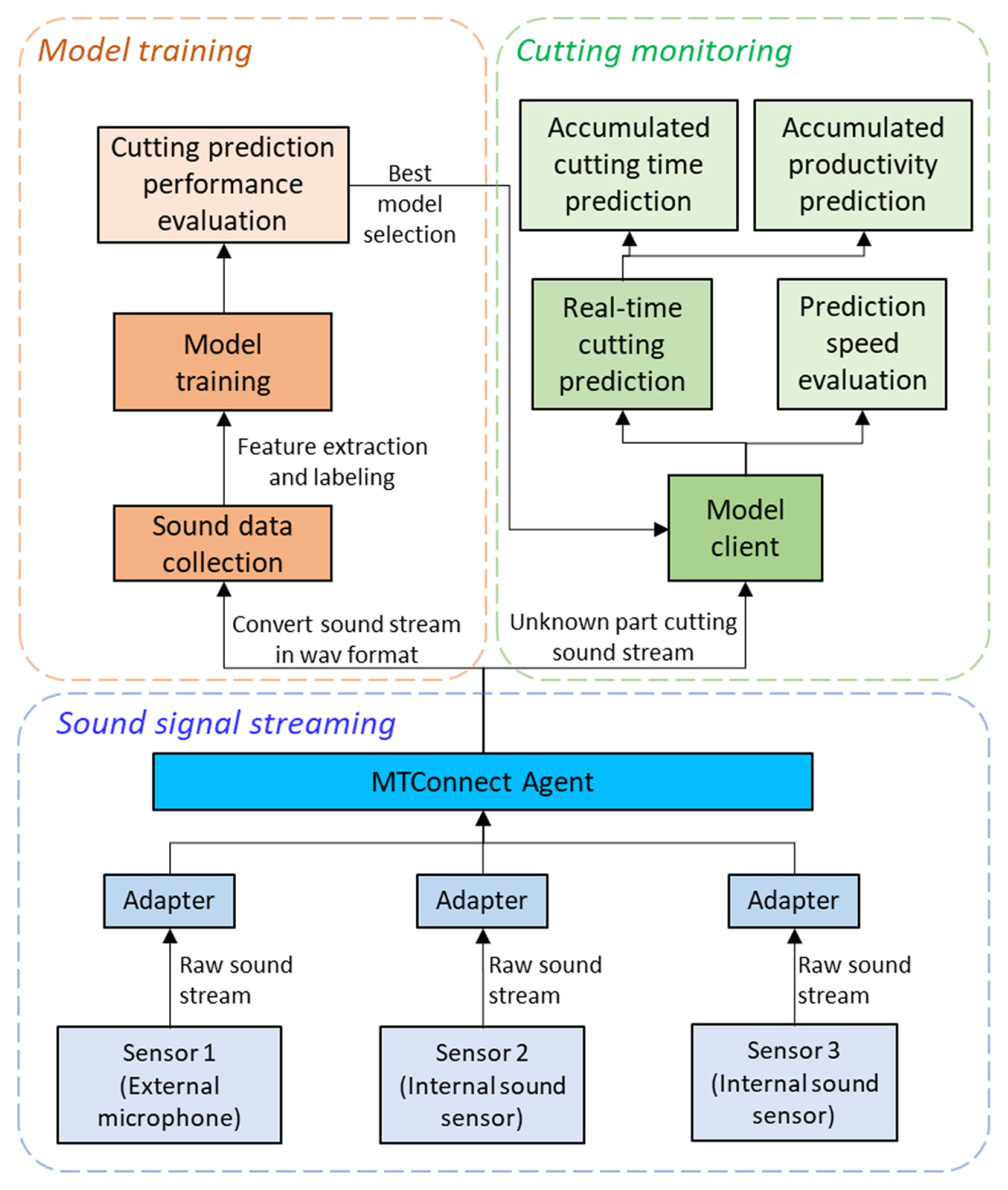
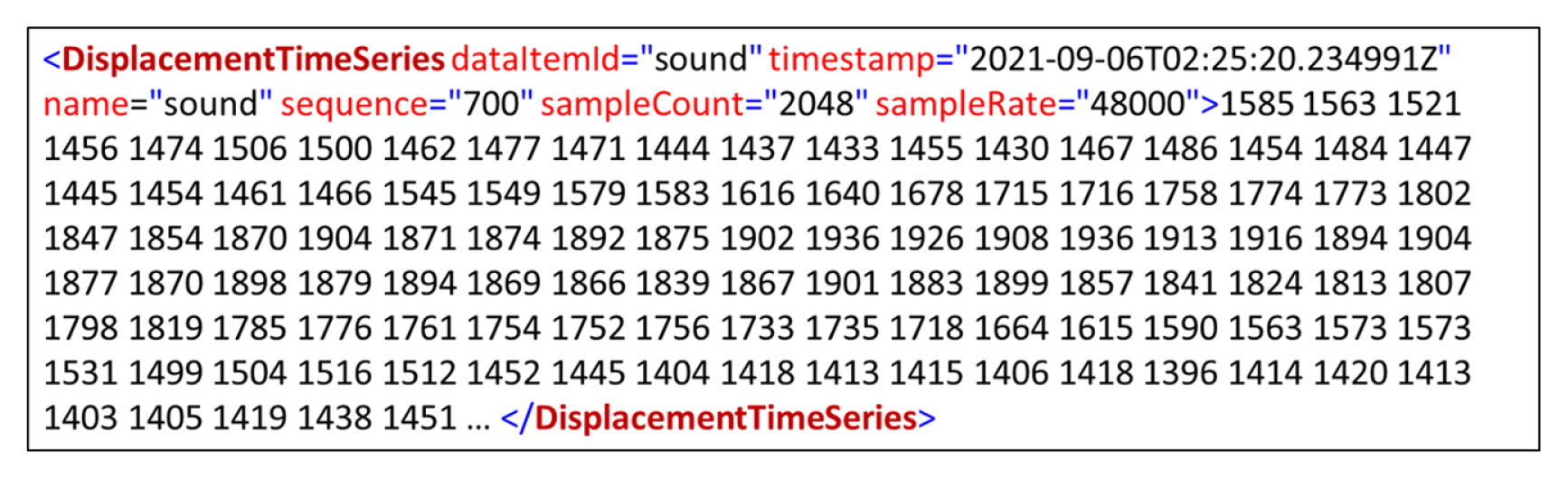
The framework of the proposed method is illustrated in Fig. 6, which breaks down into three main parts: Sound signal streaming, Model training, and Cutting monitoring. Sound signal streaming is to make raw sound data real-time buffering from the attached sensors. Model training is to train cutting prediction models based on each sensor sound signal and then select the training parameters for each sensor to achieve the best prediction performance. Cutting monitoring is to verify the trained model for unobserved and unknown part manufacturing. The selected best model for a sensor is applied to the model client in cutting monitoring in real-time for the unknown parts manufacturing that has not been trained before. To enable buffering of high sampling rate and real-time sound streams from each sensor, another MTConnect agent run by the edge computer was adopted by using Displacement representation and TimeSeries type of MTConnect standard [29]. An MTConnect adapter application to stream sound signals from the sensors was written in Python using Advanced Linux Sound Architecture (ALSA) and PyAudio module. Fig. 7 shows a sample of MTConnect DisplacementTimeSeries from a sound sensor. It contains sound data in 48 kHz sampling rate with 211 chunk size and 16-bit depth resolution of the mono-channel.
In other words, each sample contains 2,048 sound sensor data points, which have 42.67 msec length. Each data point in a DisplacementTimeSeries sample is delimited by a space at an equal time interval. The timestamp of MTConnect is the exact time of the last observation. Therefore, the timestamp of each sound measurement is tracible.
To collect sound data in an application, XML parsing, appending each DisplacementTimeSeries data, and converting them into 16-bit integer arrays are sequentially performed and then saved as a standard audio file, the WAV format, in a specific length. Because MTConnect agent takes incoming data stream as a queue sequence, ordering data in the sequence order keeps the order of incoming sound data. One of the controller data from NC is the numerical control (NC) code program name. Since different parts have different NC codes, it was able to know how many times the machine was operated for a part. However, it does not guarantee the productivity of the part because mostly several dry runs without feeding the tube bar are performed whenever the NC code is changed, or the setup is changed to ensure safety and operation. Moreover, if an operator runs the machine in the manual mode, the operational information is not logged in the controller. The collected sound data was labeled between cutting ŌĆ£ONŌĆØ or ŌĆ£OFFŌĆØ state by comparing collected NC code, actual cutting time for a specific part, and even listening sound. With the labeled sound data, CNN models were trained. To evaluate the performance of cutting prediction, data used came from new parts that were not included in the training set.
In cutting monitoring, the cutting prediction performance in terms of prediction speed in the edge computer was also performed by calculating time delay by real-time data pulling, signal processing, and the calculation of the trained model. All the tests were conducted during real production without additional experiments in order to avoid interrupting production. Details of feature extraction, labeling, and the training model are described in the following sections.
3.2 Feature Extraction
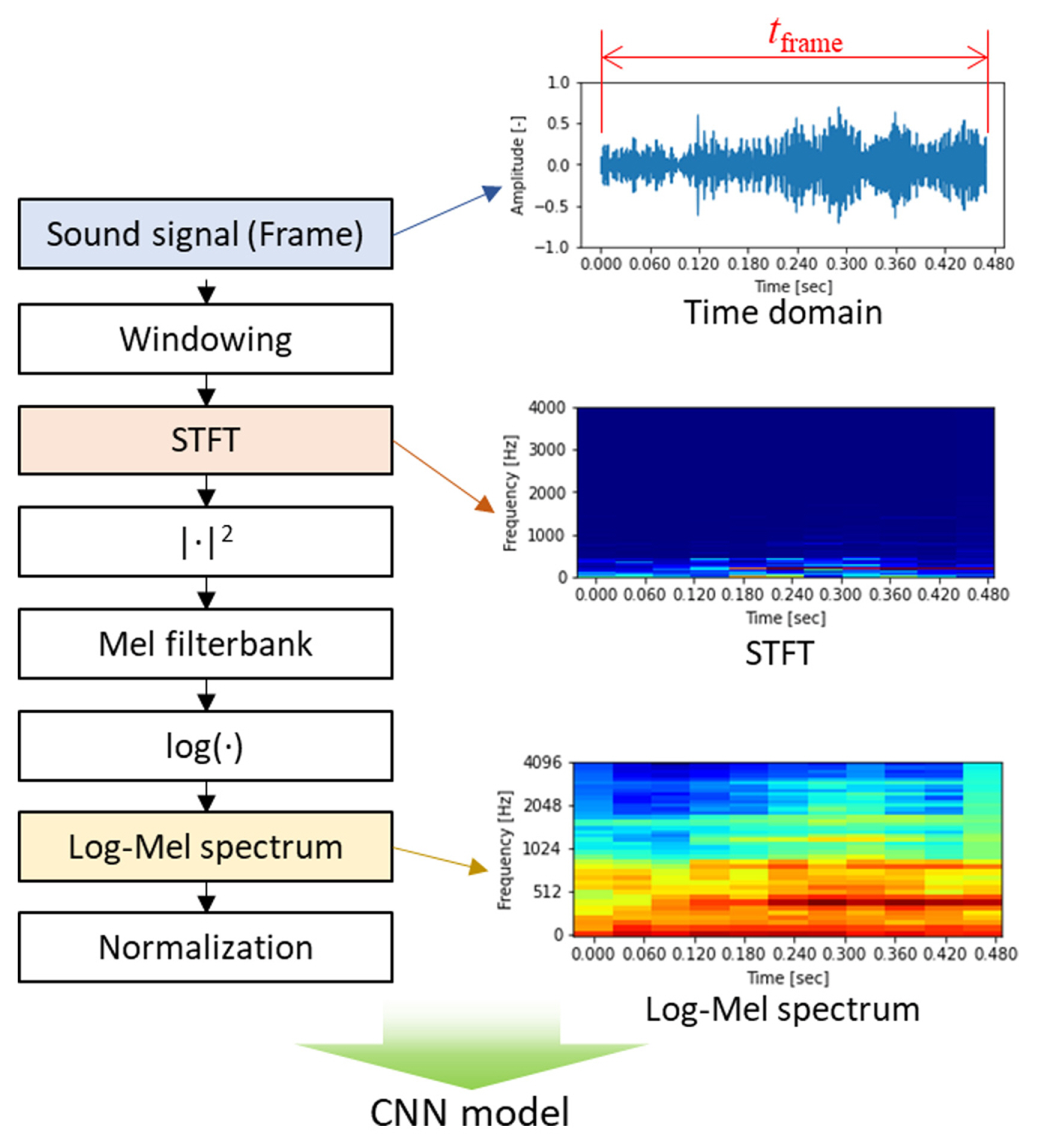
Based on the literature [21,30,31], we adopted the normalized Log-Mel spectrum as a feature for the networks. Li et al. [30] show that the Log-Mel spectrum feature has the best accuracy performance among other feature extractions in CNN for environmental sound detection. The Mel-scale is a human perceived frequency of a pure tone to its actual measured frequency. Humans are much better to tell small changes at low frequencies than at high frequencies. Mel spectrum is more suitable for human auditory sensing that indicates the linear distribution under 1,000 Hz and the logarithm growth above 1,000 Hz, which result in many ASRs adopt the Mel-scale as a step of feature extractions [32]. The workflow of feature extraction and sample visualizations of a 0.5-second length frame from sensor 2 when cutting is engaging are shown in Fig. 8.
The collected sound signal is firstly divided into time frame (tframe). We adopt the time frame as a variable of this cutting monitoring system. The range of the time frame variables is from 0.25 to 1-second in this study. Because the length of the time frame includes time information and changes the size, it affects the model training, performances, and the calculation load at edge computing during cutting monitoring. For instance, as the short time frame contains less information, not only data pulling time from MTConnect stream but also signal processing time is reduced compared to the long time frame. In terms of prediction accuracy performance, however, it is expected that the longer time frame is better than the shorter one because it contains more information. When pulling sound data stream out from the MTConnect agent, it is required to request the data as many as the sequence number which is an integer. The relationship between the frame sequence number integer (Nframe) and the length of time frame (tframe) in the unit of second is expressed as Eq. (1)
where constants, Nchunk (2048) and fs (48,000 Hz), are the sound chunk size, and the sampling rate, respectively. Because the frame sequence number is taken by rounding down, the real time frame is shorter than the target. The frame time size (tframe), the real frame time size (tframe, real), the frame sequence number (Nframe), and the number of data points in a frame as variables for the system are shown in Table 3. After framing, STFT is performed with Hamming window. The length of FFT is the chunk size, 2048, and 50% overlapped frames are used. The power spectrum, which is the square magnitude of the STFT, is also calculated.
As a Mel filter bank, 40 filter banks were adopted to calculate Mel-spectrum. The lower limit of the Mel filter bank was 20 Hz which is the lower limit of the USB microphone. The upper limit frequency is assigned as 4000 Hz. The relationship between Mel and frequency is shown in Eq. (2)
where M and f represent Mel and frequency, respectively. The Mel filter banks are expressed in Eq. (3)
(3)
where m is the number of filters and f(┬Ę) is a list of m+2 Mel-spaced frequencies. After applying the filter banks to the power spectrum of the signal and then taking the logarithm, the Log-Mel spectrum is obtained, which is denoted by LM as Eq. (4) [31].
where |X (k)|2 and k are the power spectrum in the kth point and the point of FFTs, respectively. Lastly, normalization between 0 and 1 is performed to be ready to feed into the CNN model.
3.3 CNN Model
CNN models have been widely applied for sound recognition and classification tasks [30,33,34]. CNNs are a type of multi-layer neural networks that typically contain convolution layers, subsampling layers, and fully connected (FC) layers. Even if the networks are complex because of a large amount of connectivity, the use of shared weights within layers helps in reducing the number of parameters that should be trained [35]. Parameter sharing makes CNNs greatly reduce the number of unique model parameters and significantly increase the size of the network without requiring corresponding increase in training data [36].
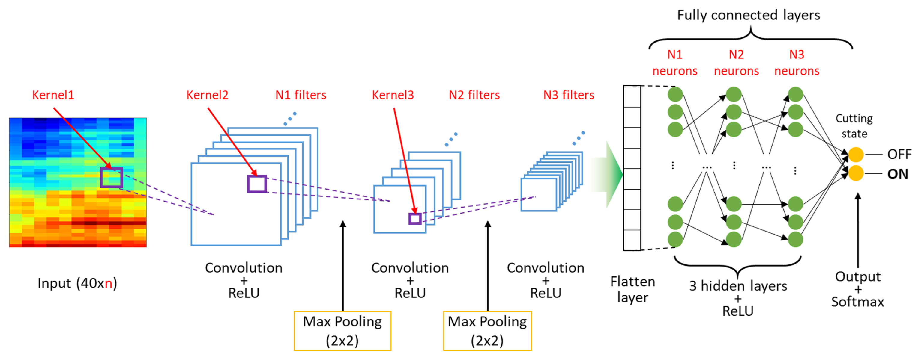
For the cutting monitoring of the tube cutting machine, we adopted 2D CNN. The CNN model architecture in this study is illustrated in Fig. 9. Because the frame time size is a variable for the model, the input size is (40 ├Ś n) where n is the second size of the 2D input feature. We selected three convolutional layers, two max pooling layers after the first two convolution layers using a (2 ├Ś 2) kernel and a stride of 1, and three hidden layers. After each convolution layer and hidden layer, rectified linear unit (ReLU) was selected as an activation function. The output layer finally has two classes, cutting ŌĆ£OFFŌĆØ and ŌĆ£ONŌĆØ. The Softmax regression was employed as a classifier of the output layer. The Softmax regression classifier predicts the class, ┼Ę, with the highest estimated probability as Eq. (5).
where K, x, and w are number of classes, feature vector, and weight vector, respectively. The Softmax classifier predicts a single class for input. The sum of the classifier is 1. As a cost function for the training model, the categorical cross entropy was adopted. Because the number of classes for the output layer is 2 (K=2), the cross-entropy cost function is equivalent to the logistic regression cost function, J, as Eq. (6).
where N is the number of input samples, y is the actual output, and p╠ä is the predicted probability. Finally, when monitoring, the trained CNN model determines the cutting state ŌĆ£OFFŌĆØ or ŌĆ£ONŌĆØ based on the input feature. In CNN, hyperparameters such as the number of filters, kernel size of convolution, and so on significantly affect the time and memory cost of training as well as prediction performance [36,37]. For hyperparameter tuning, random search was used which generally converges faster than grid search [38]. The hyperparameters for random search are summarized in and shown in Fig. 9. The order of layer number is from the input to the output. The stride of each convolution layer is 2 with zero padding. Details of the training and evaluation are described in the following section.
4. Dataset and CNN Training
4.1 Cutting Signal and Labeling
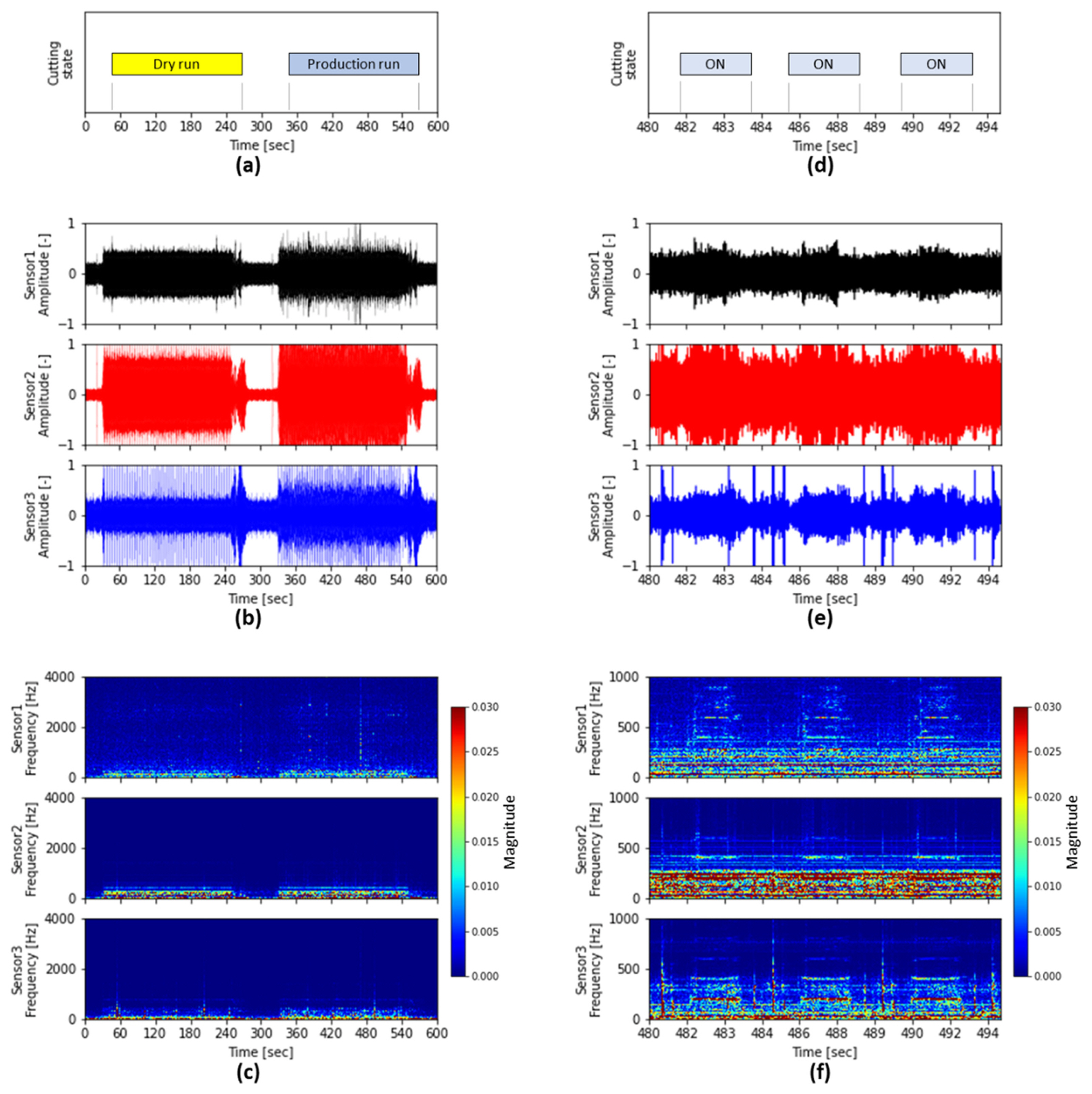
Sample sound signals from three sensors are visualized in Fig. 10. The left side plots (Figs. 10(a), 10(b) and 10(c)) are for 10 minutes to compare sounds at dry-run and production run, whereas the right plots (Figs. 10(d), 10(e) and 10(f)) are for 15 seconds of the left sound signal from 480-second to 495 second to figure out the cutting sound in detail. Both the plots are respectively aligned vertically with the time-axis so that sound signals can be compared with respect to sensor and domain. Top plots (Fig. 10(a) and 10(b)) show the cutting state according to time. Fig. 10(a) shows executing a dry run and a real production run. Other than the dry run or the production run, all the other state is idle. This is a typical example of testing as a dry run of NC code before starting real production. In the sound signal plots (Figs. 10(b), 10(c), 10(e), and 10(f)), subplots of signals from sensor 1, sensor 2, and sensor 3 are placed from the top to bottom. It is observed that the amplitude of sound signals when cutting tube bar is increased in Fig. 10(b) if compared between dry run and production run. In addition, idle sound signals are distinct. Fig. 10(e) shows three times cutting events in the time domain. The cycle time is 3.9 seconds and the cutting time in each cycle is approximately 1.97 seconds. As cutting is being engaged, the amplitudes of sound signals also increase. Fig. 10(c) shows STFT spectrogram of the entire signals. The frequency range in Fig. 10(c) is from 0 to 4,000 Hz. Signal magnitude higher frequencies above 1,000 Hz are weaker than the lower frequency range. Note that Fig. 10(f) shows STFT spectrogram of frequency range from 0 to 1,000 Hz to see low frequency components in cutting. It is difficult to clarify the cutting start from the time domain in Fig. 10(e) whereas cutting start time as well as cutting signals are recognizable in the time and frequency domain in Fig. 10(f). It shows sounds emitted by cutting engagement are perceptible by humans.
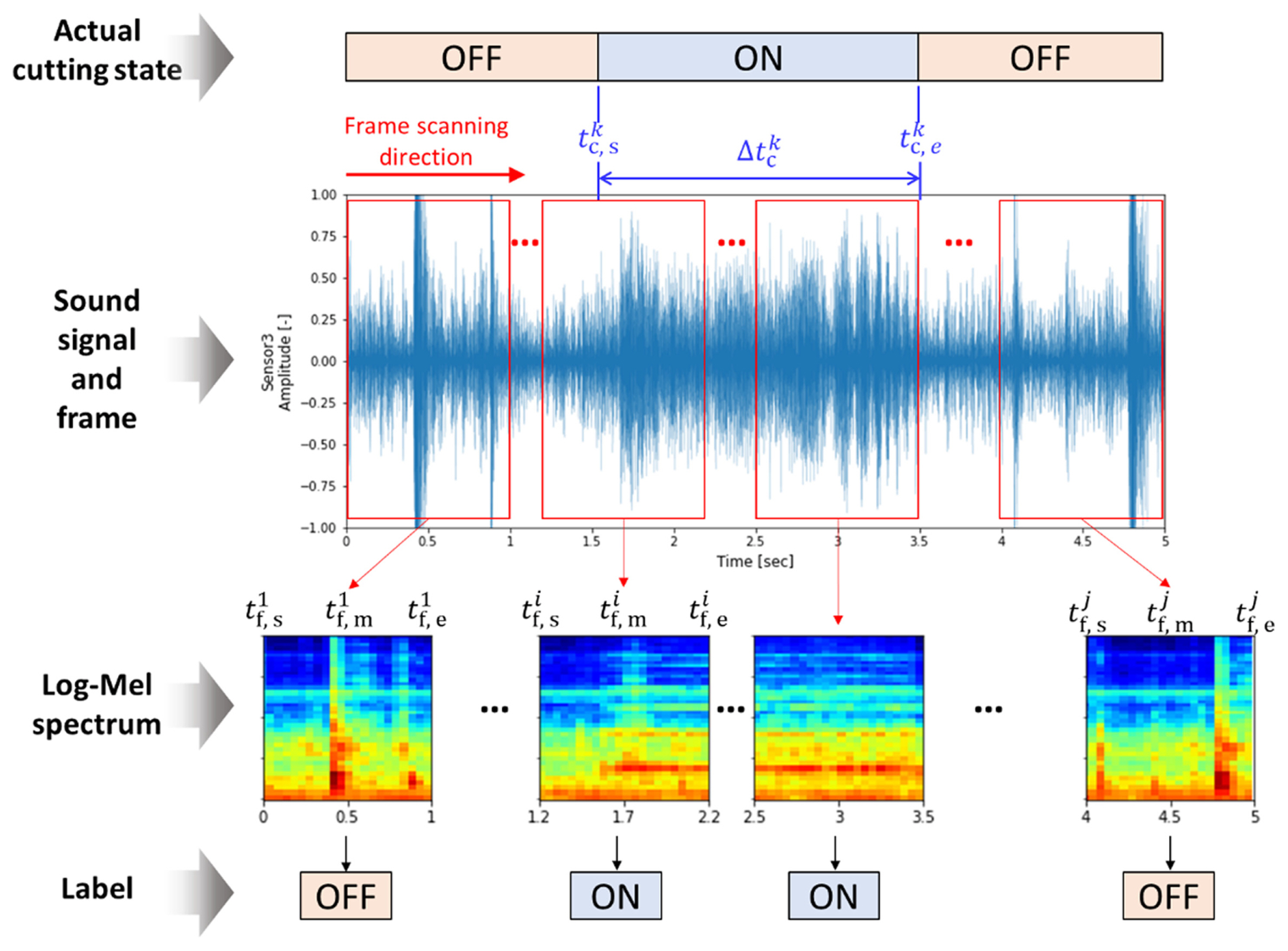
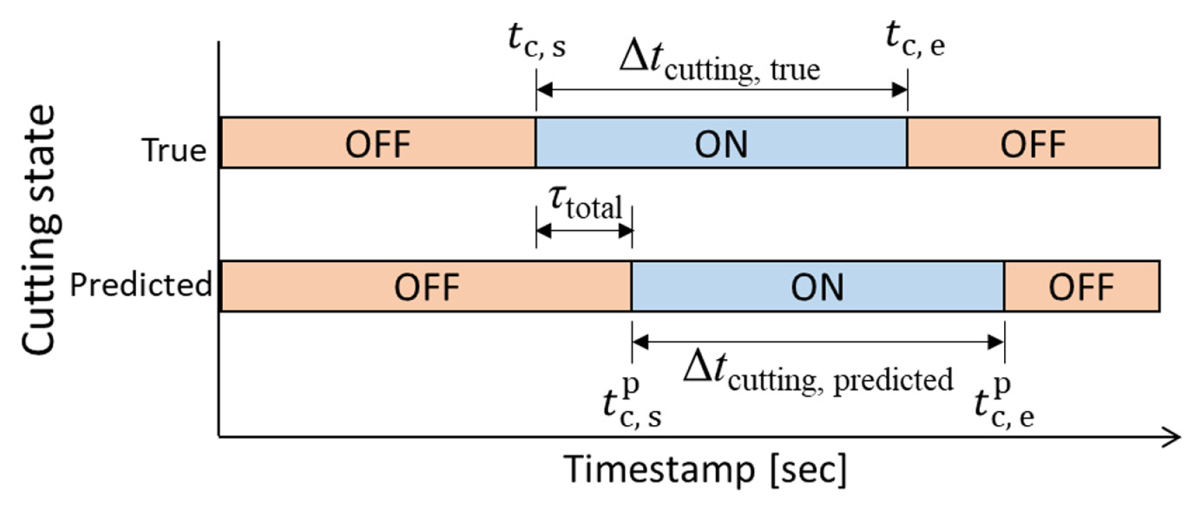
The labeling procedure to generate training and evaluation datasets is illustrated in Fig. 11. In the tube cutting process, a subprogram NC code is run every cutting cycle. Thus, subprogram NC code timestamps from MTConnect data of the PLC were utilized to determine the actual cutting start time and cutting end time. The actual cutting start and end timestamps are denoted by tc,s and tc,e, respectively. However, it was required to confirm actual cutting by listening to sound or visualizing the collected data because dry run happens occasionally as Fig. 10(a), especially when the NC code is changed. The cutting time per part, Δtc, in this example, is approximately 1.97 seconds. Based on the timestamps of the actual cutting start and end, labeling was performed as Fig. 11.
As discussed in the previous section, the collected sound data were split into a set of time frames by scanning the entire collected sound files. The step between time frames when scanning is 2048 because the sound chunk size Nchunk, is 2048 that is the step having a 42.67 msec interval. Each time frame, tframe, is processed to generate an input which is a Log-Mel spectrum. Therefore, each Log-Mel spectrum input contains time information. Let the start and end timestamps of the ith time frame be
t f , s i t f , e i t f , m i t f , s i t f , e i
To verify the effect of the size of the time frame on cutting state prediction performance, four different lengths of time frames were selected as noted in Table 3. Fig. 11 shows an example of the 1-second time frame size. The first time frame is between 0 and 1 second. The cutting starts at 1.52 seconds and ends at 3.48 seconds. Therefore, the first time frame in Fig. 11 has ŌĆ£OFFŌĆØ label. The ith time frame in Fig. 11 has ŌĆ£ONŌĆØ label because the middle timestamp is bigger than the actual cutting start timestamp and less than the cutting end timestamp. This procedure was performed for all training and evaluation datasets. After finishing scanning for each time frame size, the labels and the corresponding input features are fed into training the CNN model.
4.2 CNN Training
While in real manufacturing, more than two weeks of both sound data and NC data were collected. For training and evaluation datasets, the manufactured data at 8 different parts were selected. Each data within training and evaluation datasets is different due to either change of part design or material, which leads to different cycle times and cutting sounds. Table 5 summarizes the training and evaluation datasets. In Table 5, the alphabet names of parts were arbitrarily given. In the training dataset, dry run or idle data were also included considering an application to real manufacturing.
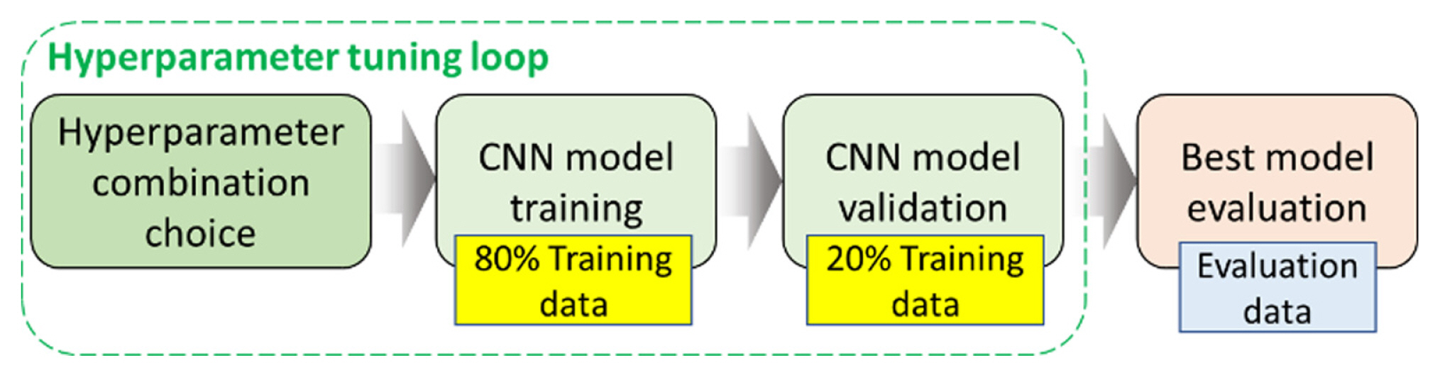
Python and TensorFlow were used for CNN model training. CNN model training using hyperparameter tuning and the evaluation procedure is illustrated in Fig. 12. Details of the CNN model and the hyperparameters are described in section 3.3. Ratios of training and validation data in the hyperparameter search loop were 80% and 20% of the training dataset, respectively. The number of trials for the hyperparameter combination was chosen to 100. Networks of each combination were trained with 30 epochs, and 512 batch sizes. The Adam optimizer was used with a learning rate 10ŌłÆ4. The validation accuracy was the metric to select the best combination of the hyperparameters. After 100 trials, the best model was trained again using the training dataset up to 50 epochs. Finally, the trained best model was tested using the evaluation dataset.
5. Result and Discussion
5.1 CNN Training Results
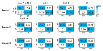
The shapes and number of network parameters of the best models according to the sensors and the size of time frames are summarized Appendix 1. The number of the parameters of the CNN models increases as input feature size increases. All confusion matrixes on both the training and evaluation datasets are in Appendix 2.
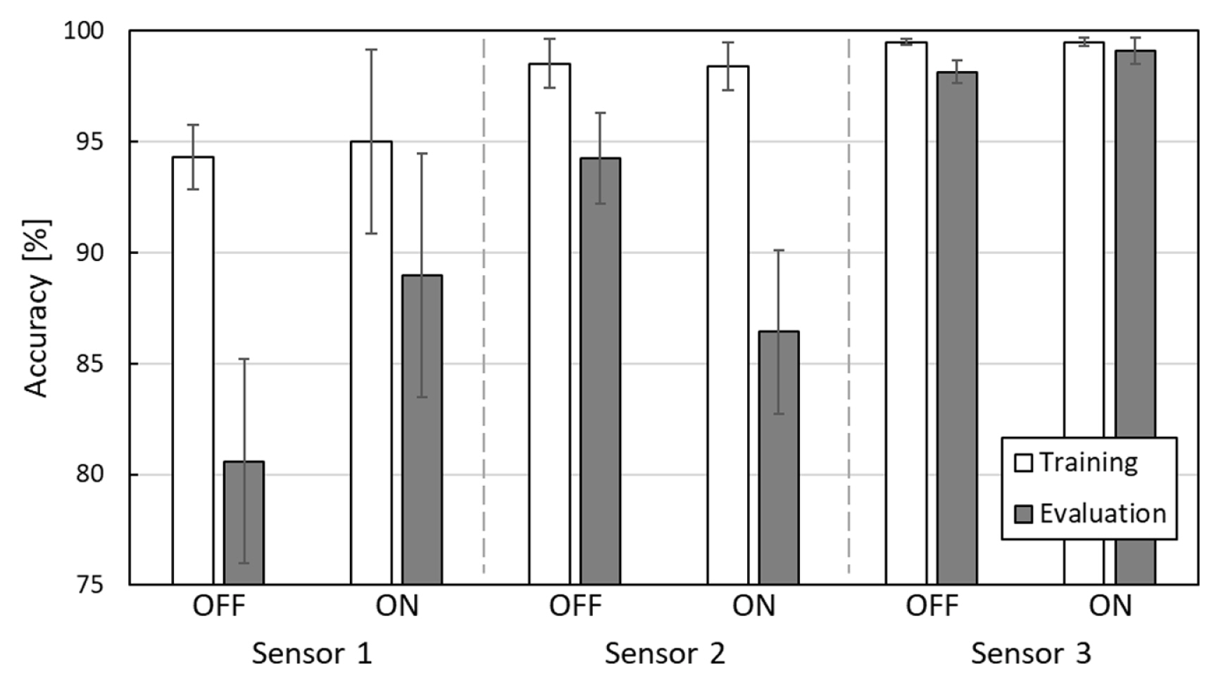
Fig. 13 shows the averaged accuracy metrics on sizes of the time frames to see the prediction performance of the CNN model by sensors. The error bar is the standard deviation of all the sizes of the time frames. Sensor 3 showed the best prediction performance in terms of model accuracy whereas sensor 1 showed the worst on both training and evaluation datasets. In the training dataset, all sensors showed both cutting ŌĆ£OFFŌĆØ and ŌĆ£ONŌĆØ accuracy higher than 90%. Factory noise from other machines perhaps caused the results because the data was collected in real manufacturing on the shop floor. Other than cutting sound, sensors 1 and 2 compared to sensor 3 capture not only sounds from other components of the machine but also noise from other neighboring machines, which is shown in Fig. 10(f). In other words, one challenge of machine sound monitoring is the factory noise by which airborne sound monitoring is mostly affected. The models of sensor 1 mostly predict false positives when neighboring machines are operated or when loud noise is generated. This leads to poor prediction performances compared to the other sensors. Another challenge is that false predictions frequently occur at the very start and end of cuttings although this is inevitable. Since the labeling algorithm determines the cutting state ŌĆ£ONŌĆØ if the model input contains cutting signals more than half of the frame length, in some cases the time length difference between cutting signals and non-cutting signals in the time frame is even less than 10 msec. However, this does not significantly affect the prediction performances overall. If a cutting time per part is 3 seconds, there are 70 successive model inputs which have to have true ŌĆ£ONŌĆØ labels. If a single inference is wrong at the very start or end of the cutting, the accuracy is approximately 98.6%. It has been studied that increase in the size of training datasets and data augmentation methods are able to improve the prediction performances of sound classification models [39]. Adding background and factory noise is one way of data augmentation of sound [40]. Generative adversarial networks (GANs) are also sophisticated means for data augmentation using deep learning to improve sound classification performances [41,42].
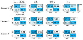
In all sensors, the model accuracy on the evaluation dataset was worse than on the training dataset. This results from the evaluation datasets are untrained manufacturing data as well as a much larger size than the training datasets. Especially, the entire size of the training dataset was 7 minutes while the size of the evaluation dataset was 4 hours. When it comes to the prediction performance of the generalized cutting state of the tube cutting machine, however, all models show higher than 80% of prediction accuracy. The models by sensor 3 regardless of the time frame sizes result in higher than 98% of prediction accuracy in both training and evaluation datasets.
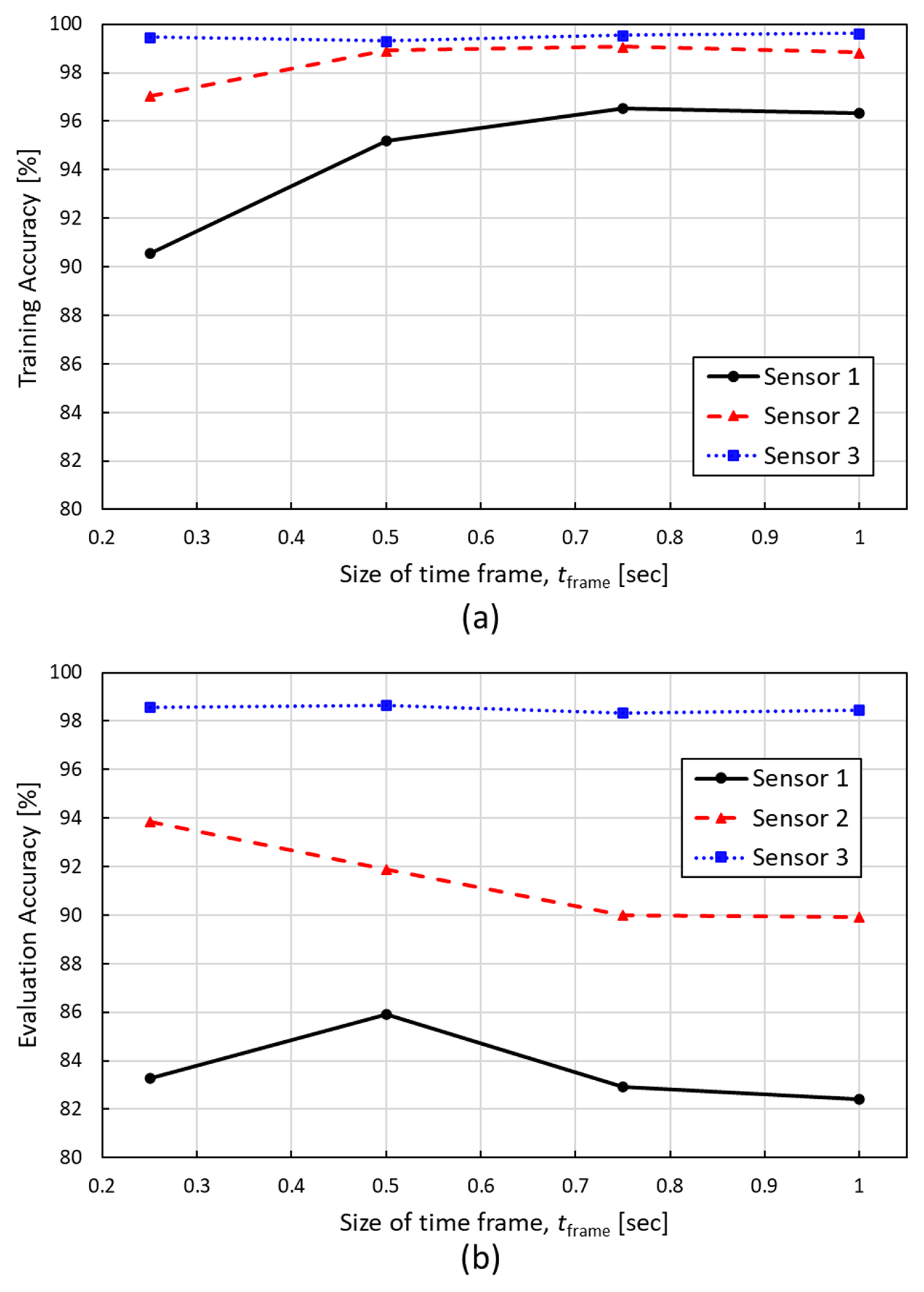
Figs. 14(a) and 14(b) show the overall model accuracy of all classes according to the size of the time frames on the training dataset and the evaluation dataset, respectively. The results of the training dataset in Fig. 14(a) show that the size of the time frame hardly affects model accuracy on sensor 3. Model accuracies of sensor 3 on the training dataset were from 99.33 to 99.64%. On the other hand, model accuracy was improved on sensors 1 and 2 as the number of sizes of the frame increased. From the results of the evaluation dataset in Fig. 14(b), sensor 3 shows the highest model accuracy in all sizes of time frames. However, the 0.5 s time frame size showed the highest model accuracy in sensor 1. In sensors 1 and 2, on the other hand, the increase in the size of time frames shows lower trend in the model accuracy on the evaluation dataset.
5.2 Productivity Prediction Performance Evaluation
To evaluate the CNN models in respect of the accumulated cutting time and productivity predictions, The best CNN model was simulated according to each sensor and each size of time frame. For the simulation, the evaluation dataset was used. First, the evaluation dataset, the WAV format sound file, for each sensor was split by each frame size. And then, the CNN model was applied to the split data sequentially from the first frame to the last frame. Based on the predicted results from the model, the accumulated cutting time error ecutting was calculated. The cutting time error is defined as Eq. (8).
where Tcutting is accumulated cutting time, which was calculated by multiplying real cutting time per part and the number of manufactured parts, and i, n, and y are the frame number from 1, the number of frames, and the output of the CNN model, respectively. In the simulation, each CNN model output which is ŌĆ£OFFŌĆØ or ŌĆ£ONŌĆØ continues for the time step Nchunk/fs ( Ōēģ 42.67 msec). Therefore, by multiplying the number of ŌĆ£ONŌĆØ outputs and the time step in all frames, it was able to predict the accumulated cutting time for each model. To evaluate the performance of productivity prediction, the part counting error epart count is defined as Eq. (9).
where Npart is the accumulated part count and
n p a r t i
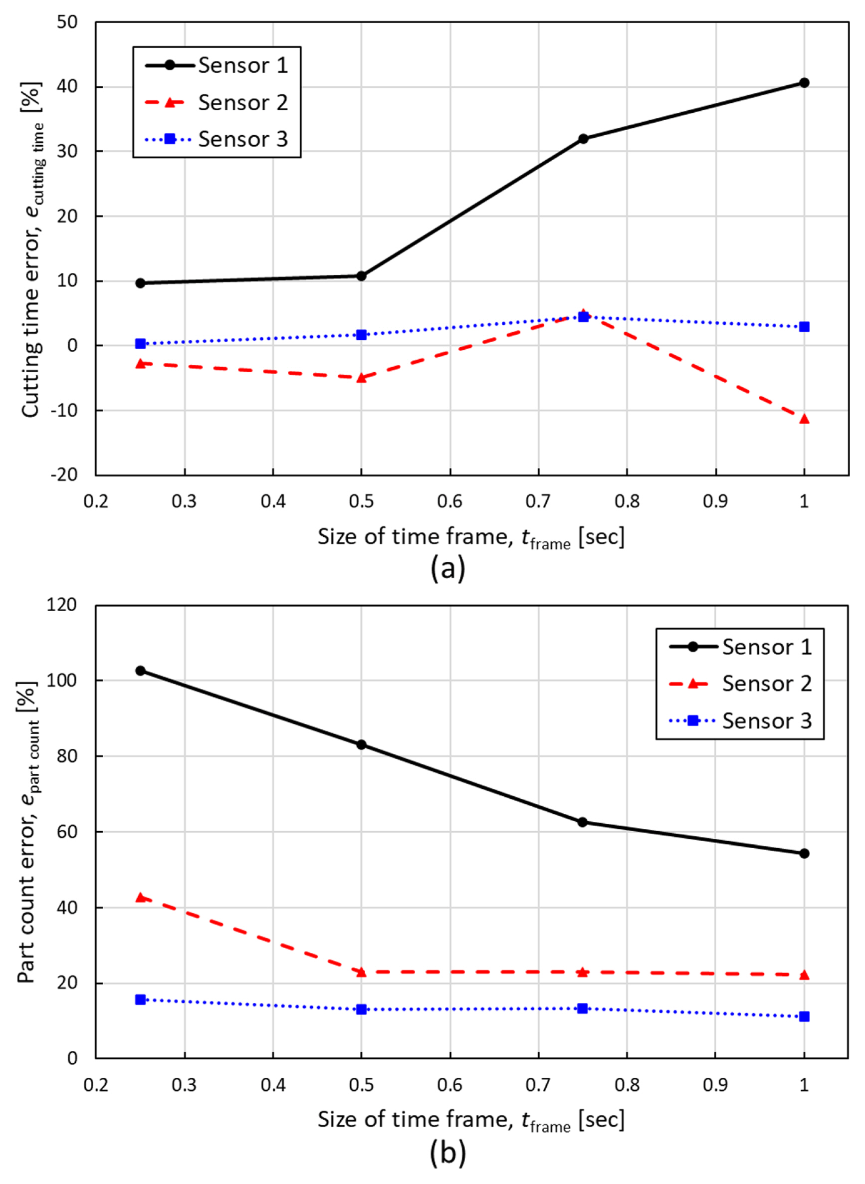
Figs. 15(a) and 15(b) show the cutting time prediction error and the part count error according to all sensors and sizes of time frames. As the size of time frames increases, the cutting time error was bigger. In all sensor cases, the minimum cutting time errors were 9.71, ŌłÆ2.76, and 0.36% for sensors 1, 2, and 3, respectively, when the size of time frames was 0.25-second. Contrarily, when the size of time frames was 1-second, the cutting time prediction error was the biggest in all cases, and the results were 40.57, ŌłÆ11.2, and 2.99%, respectively, for sensors 1, 2, and 3. However, the part count prediction error showed opposite results from the cutting time error; as the size of time frames increases, the part count error was reduced for all sensor cases. The part count errors in case the size of time frames was 0.25-second were 102.6, 42.7, and 15.7% for sensors 1, 2, and 3, respectively. On the contrary, the part count errors in 1-second time frames were 54.4, 22.3, and 11.3%, respectively.
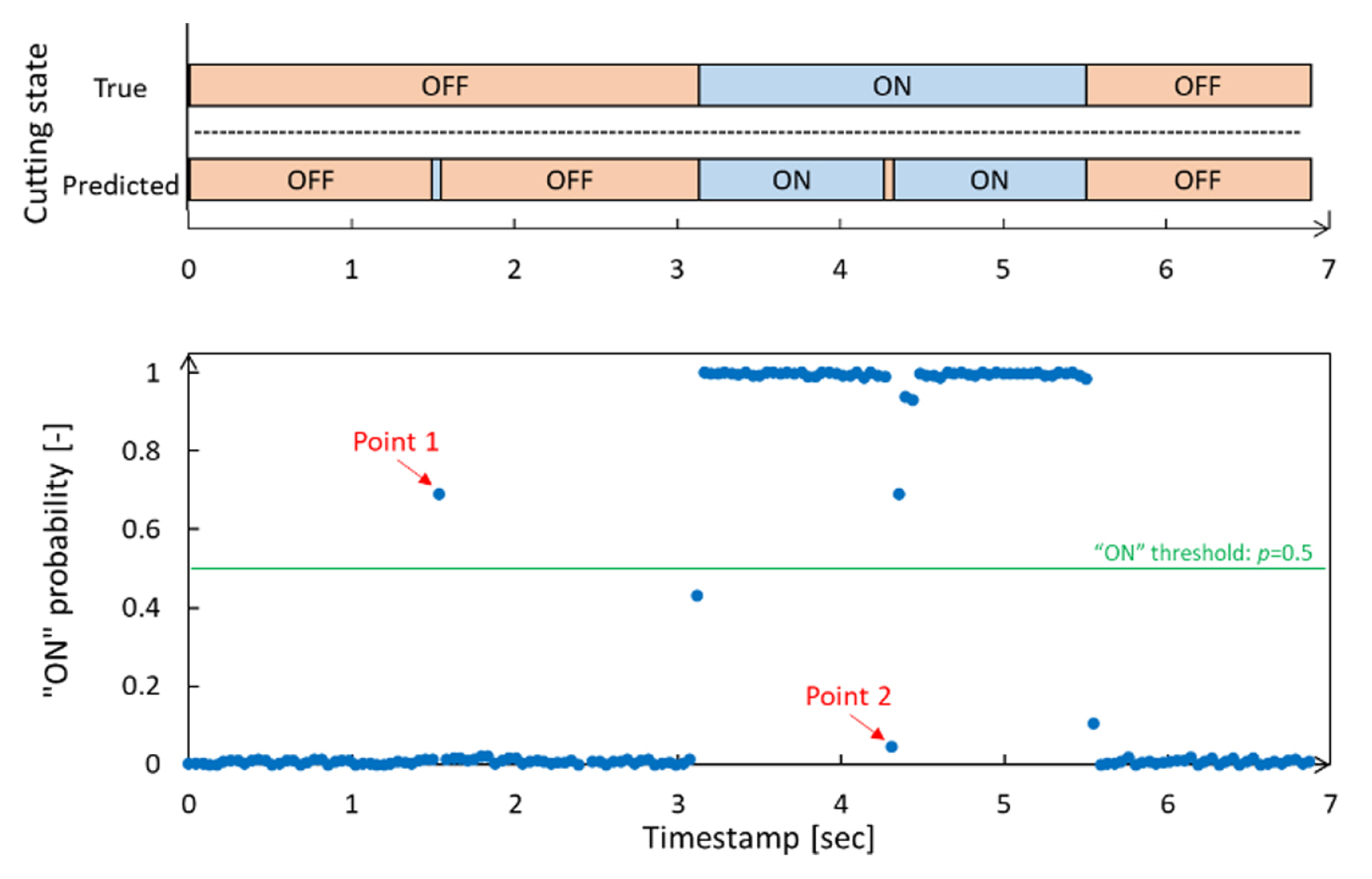
Overall, the part count errors are all positive and large compared to model accuracy and the cutting time error. This is because every change in the output of the model is reflected in part count as Eq. (10). For instance, a part that has a 1-second-long cutting must contain at least consecutive 22 of the ŌĆ£ONŌĆØ states. If one false prediction happens during a single cutting, it causes not one count but two counts. On the other hand, a single false positive prediction in consecutive true ŌĆ£OFFŌĆØ states, occurs with one error part count. Fig. 16 shows samples of the results from the simulation of sensor 1 with the 0.75-sec length of time frame. Cutting state results in both true and predicted according to timestamps are on the top. The ŌĆ£ONŌĆØ probabilities according to the timestamps are at the bottom. Both graphs have the same timestamp range. Because this model has two classes and the Softmax is used for output node activation in case that the ŌĆ£ONŌĆØ probability is more than a threshold of 0.5, the output is ŌĆ£ONŌĆØ. At point 1 of Fig. 16, the true cutting state is ŌĆ£OFFŌĆÖ but the model determined ŌĆ£ONŌĆØ. This error is small in terms of cutting time because each point has 42.67 msec duration, but it causes one false part count. Further, at point 2, the true cutting state is ŌĆ£ONŌĆØ while the model determined ŌĆ£OFFŌĆØ even if that point is in the middle of cutting. This also makes one more part count error. It is a limitation of the proposed method. Although it is accurate for predicting cutting time, it would not be perfect, especially in the circumstance of productivity prediction is important. To overcome this limitation, an additional algorithm is required to determine whether actual cutting happens or not. An additional algorithm that determines positive or negative predictions to be reflected in the part count would help to improve the part count prediction performance. For example, adding a rule of a minimum number of successive ŌĆ£ONŌĆØ or ŌĆ£OFFŌĆØ inferences prevents false part count predictions as in Fig. 16. In addition, it is also possible to apply a hybrid model with the Gaussian mixture-model (GMM) [30] and the hidden Markov model (HMM) [33], or long-short term memory (LSTM) [43], which have been widely utilized in sound event recognition.
5.3 Real-Time Monitoring Performance
The proposed method and the best CNN models were applied to real-time cutting state monitoring while real manufacturing is in progress to verify how fast the model predicts the cutting state and how accurate the cutting time per single part is. The cutting time and the time delay in real-time monitoring are shown in Fig. 17. Cutting time Δtcutting is defined as time differences between start time and end time during cutting. The cutting time error per part ecutting single is defined by Eq. (11).
The time delay is defined as time differences between true and predicted cutting start time. As proposed in Fig. 4, edge computing was employed. The hardware and software for monitoring are summarized in Table 6. To run the CNN model on Raspberry Pi, we tried both TensorFlow and TensorFlow Lite modules to compare model response rate. When monitoring, each sensor, each size of time frame, and each model were applied for 10 minutes to evaluate the real-time monitoring performance. The true average cutting time per part during the test was 3.04 seconds. While the monitoring process is working, raw sound signals were also collected at the same time to confirm the performance.
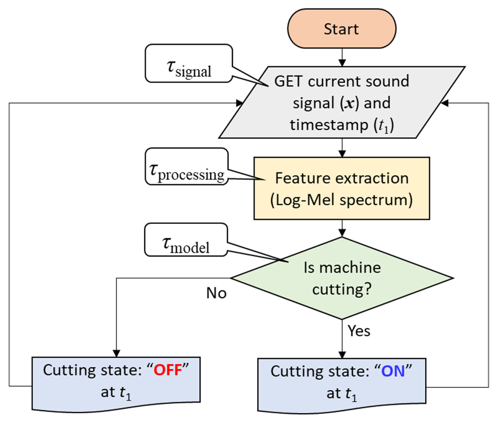
The algorithm of monitoring cutting state is illustrated in Fig. 18, which is divided into three steps. First, the program requested sound data from the time frame (tframe) before to the current and append all chunks into a sound array. Second, the signal was processed to the Log-Mel spectrum as feature extraction. Lastly, the feature was fed into the CNN model to determine the cutting state. These three steps were repeated until the program was halted. The taken time for each step was denoted by Žäsignal, Žäprocess, and Žämodel, respectively. The total taken time, namely the total time delay Žätotal, was calculated by adding all time delays of the three steps in the algorithm. Because the computing time is not affected by sensor type, the results of each size of the time frame were averaged from all sensors.
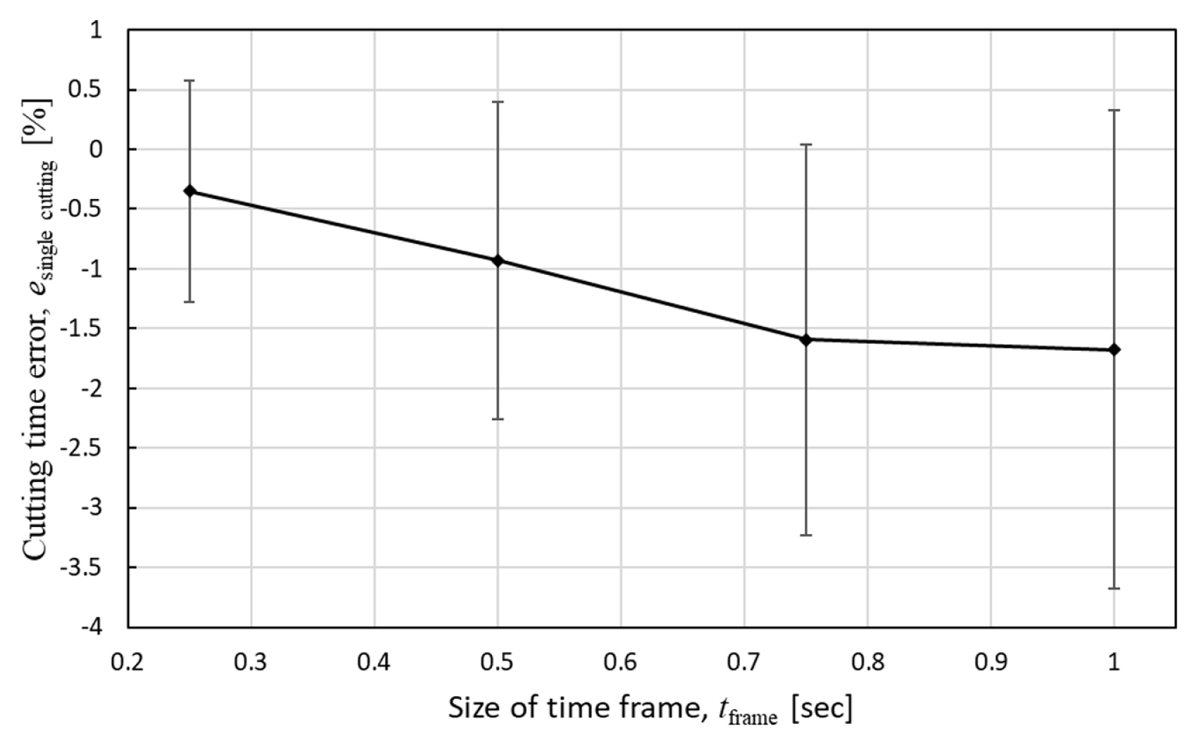
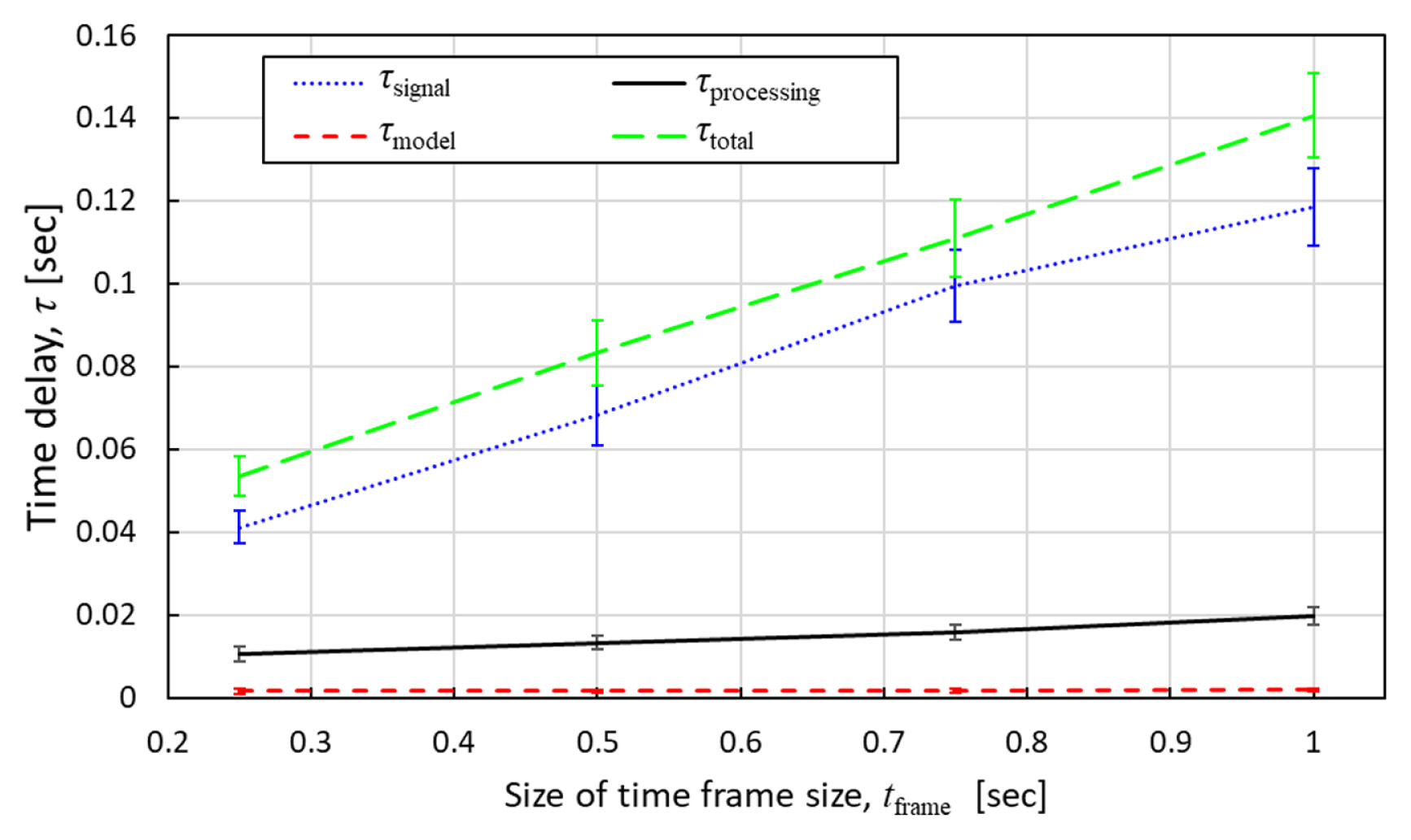
Fig. 19 shows the results of the cutting time error per part according to the size of the time frames in the percentage unit. In all sizes of the time frames, the predicted cutting time per part was shorter than the actual cutting time. The minimum error was ŌłÆ0.5% in the case of the 0.25-second time frame. As the size of the time frames increases, the cutting time difference per part and the variation were bigger. The monitoring time delay measurements according to the size of the time frames are shown in Fig. 20. Among time delay factors, the time delay Žämodel by the CNN model run by TensorFlow Lite, averaged 1.7 msec, was the shortest, and it was barely changed by the size of the time frames. In case the CNN model is run by TensorFlow, the averaged time delay was 123.6 msec which is 73 times slower than TensorFlow Lite on Raspberry Pi. The processing time delay Žäprocessing to convert raw sound signals to the Log-Mel spectrogram was the second short. Even though the processing time delay was increased as the size of the time frames increased, the amount of increment was small. The processing time delay was 11.76 msec in the 0.25-second time frame, and 20.57 msec in the 1-second time frame. The most dominant contributor to the total time delay was the signal time Žäsignal. The delay time increment according to the increase of the size of the time frames was also biggest in the signal time. In the case of the 0.25-second time frame, the signal time delay was 41.16 msec whereas it was 117.64 msec in the 1-second time frame. The total time delay increased as the size of the time frames increased. These time delays determine the taken time by each loop of the algorithm as well as the time differences between the cutting start times of true and predicted. The time delay results explain why the variation of the cutting time error per part was increased as the size of the time frame was increased. Because the total time delay determines the rate of the model and how fast the model is able to respond, for example, the differences and variations of cutting time are getting bigger as the time delay increases. Therefore, if the response speed of monitoring is important, the smaller time frame is the better choice.
6. Conclusion and Future Work
In this paper, a real-time cutting state monitoring for the tube cutting machine based on sound with MTConnect framework using the CNN model was proposed. An external microphone (sensor 1) on the machine enclosure and two internal sound sensors on the machine enclosure (sensor 2) and on the base (sensor 3) were deployed to compare the performance of predicting cutting state by the types of sound sensors and the locations. In addition, four different sizes of the time frame were compared in terms of the prediction accuracy of cutting state at the CNN model training as well as real-time monitoring performances. The Log-Mel spectrogram was employed as feature extraction for the CNN model. To train the CNN model, a random search was used to determine the number of filters of the convolution layers, kernel sizes, and the number of neurons of the hidden layers for each sensor and each size of the time frame. The evaluation dataset was collected during producing different parts, which was not used in training dataset to verify whether the CNN model tells unknown part cutting state.
The prediction accuracies of cutting state according to the size of time frames on the training dataset were approximately 90.6ŌĆō96.3% (sensor 1), 97.0ŌĆō98.8% (sensor 2), and 99.5ŌĆō99.6% (sensor 3), and on the evaluation dataset were approximately 83.3ŌĆō85.9% (sensor 1), 89.9ŌĆō93.9% (sensor 2), and 98.3ŌĆō98.6% (sensor 3). The smaller size of the time frames showed higher prediction performance in terms of the accumulated cutting time whereas low in terms of predicting the accumulated productivity. When it comes to sensor selection and location, the internal sound sensor on the machine base showed the best predictions in both cutting time and productivity. However, the proposed monitoring method shows a limitation on productivity prediction. Further studies on predicting productivity are required to improve the suggested framework. Real-time monitoring performances with respect to prediction speed and delay were also analyzed according to the sizes of the time frames. As the time frame was longer time delay and the cutting time errors per part were also increased. Therefore, if the monitoring response speed and the prediction accuracy of cutting time are important, the smaller size of the time frame is recommended, while bigger time frame for predicting productivity.
In future works, improving the prediction of productivity by utilizing a hybrid model or additional algorithm will be performed. The scope of monitoring for the tube cutting machine will be also extended during cutting to include condition-based monitoring (CbM) to predict cutting integrity, tool condition monitoring (TCM), and so on. Moreover, the proposed method is expected to be applied to general metal cutting machines such as CNC mills and lathes.


 PDF Links
 PubReader
 Full text via DOI
 Download Citation
  CrossRef TDM


