
 E-mail
 Print
Print facebook
 twitter
 Linkedin
 google+
List of Symbols
dn
The Minimum Distance between the Optical Fiber and the Tool
dw
The Maximum Distance between the Fiber and the Tool
Ecyc
Electric Field of the Light between the Two Mirrors on the Fabry-Pérot Interferometer
Einc
Electric Field of the Light Incident to the Fabry-Pérot Interferometer
Eref
Electric Field of the Light Reflected from the Fabry-Pérot Interferometer
ey(x)
The Straightness Error of the X-axis Guideway along Y-axis Direction
f (x)
The Profile Error from the Standard Block
J
The Imaginary Unit
l
The Geometric Distance between Reflection Surface 1 and Reflection Surface 2
L
The Distance between the Optical Fiber and the Axis of the Tool
Lw
The Distance between the Optical Fiber and the Tool Axis
n
The Refractive Index of the Medium at Wavelength of 1,550 nm
PA(x)
Raw Output of Sensor A
PB(x)
Raw Output of Sensor B
r
The Distance between the Measured Points and the Axis of the Tool
ri
The Reflection Coefficient of Reflection Surface i
rn
The Radius of the New Tool
rw
The Distance between the Tool Axis and the Point that is Closest to the Axis
s
The Radial Runout
si
The Average Coordinate along with (i = 1) and Perpendicular to (i = 2) the Fiber Axis
ti
The Transmission Coefficient of Reflection Surface i
xn
The Position of the Measured Points
(xci
yci, zci), The Cartesian Coordinates of the Geometric Center of the ith Layer to be Scanned
α
The Axial Runout
αi
The Angle between the Tool Axis and the Vertical Direction along with (i = 1) and Perpendicular to (i = 2) the Fiber Axis
λ0
The Wavelength of Light in Vacuum
λFSR
Free Spectrum Range of the Spectrum
λm
Wavelength of the Maximums and the Minimums of the Interference Spectrum with Order Number m
φ
The Phase Change of the Light when Travel in the Cavity for a Roundtrip
1 Introduction
Optical sensors such as optical interferometry have been widely applied in different areas such as environment science [1–3], biology [4–6], and engineering [7–9]. It has also been used in smart manufacturing such as high precision measurement and positioning [10,11]. Compared with traditional interferometers based on space optics, optical fiber sensors provide a more stable environment since the detection light is guided inside the fiber. Therefore, they are less sensitive to environmental disturbances such as scattering and absorption fluctuation in the air. Moreover, optical fiber sensors are compact [12–14], and therefore can be installed in limited spaces. In this paper, we use an optical Fabry-Pérot interferometer (FPI) as a displacement sensor to reconstruct the three-dimensional (3D) profile of a machine tool and measure the straight error of a computer numerical control (CNC) machine tool. An open optical fiber FPI has a simple structure and a higher finesse compared with other types of interferometers such as Michelson interferometers and Mach-Zehnder interferometer due to its resonance nature [14,15]. Therefore, it has a higher signal-to-noise ratio which makes it possible to work in non-ideal environments. Commercial interferometers usually monitor the distance based on the intensity change of a Michelson interferometer, however this method needs high precision calibration. In our previous research [16], we introduced an open optical fiber FPI that gives the optical distance between the fiber and the target directly from the interference spectrum.
In this research, we will introduce the application of optical fiber FPIs as distance sensors in smart manufacturing. First, we will introduce the basic principle of FPI and the method to reconstruct the 3D profile of a machine tool before and after being used. The spectrum quality identification method and the spectrum analyzing method will be introduced. Based on the interference spectrum of the FPI, the distance between the optical fiber and the surface of the target can be determined. To reconstruct the 3D profile of the tool, we need to fix the optical fiber while rotating the tool along its axis so that the distance between the fiber and the surface of the tool can be monitored. The distances between the fiber and points of the surface of the tool allow us to measure the profile of the tool. With the reconstructed profile, we can further calculate the runout and the tool wear of the tool. To improve the analyzing speed, different machine learning algorithms were trained to find out the distance between the fiber and the target from the interference spectrum. Then, the machine learning algorithm was applied to analyze the spectra to measure the straightness error of a CNC machine tool using the two-point method. The measurement result of the proposed method will be evaluated by a coordinate measurement machine (CMM).
2 Sensing Principle
2.1 Principle of Fabry-Pérot Interferometers
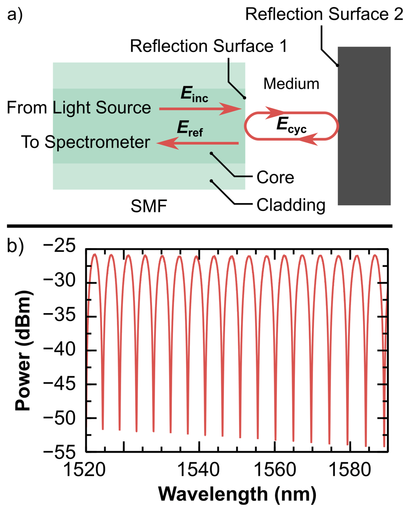
FPIs consist of two parallel reflection surfaces and the space between them. In this experiment, we used a single mode optical fiber (SMF) to form an open FPI to measure the distance between the tip of the SMF and the surface of the target. Fig. 1 (a) shows the basic working principle of the FPI we used in this experiment. Incident light Einc comes from the light source and propagate along the core of the SMF. When reaching the interface (Reflection Surface 1) between the Core and the Medium between the SMF and Target, part of light will be reflected by Reflection Surface 1 and the rest will propagate through the surface. Then, the light will be reflected by the surface of Target (Reflection Surface 2) and then reflected by Surface 1 again. Therefore, the light will be reflected between Reflection Surface 1 and 2 and resonance occurs. The structure formed by the two reflection surfaces and the space between them is called a Fabry-Pérot cavity (FP cavity).
Due to the boundary conditions of the FP cavity, light with wavelengths that are supported by the cavity will interfere constructively and therefore have higher powers. Light with wavelengths that are not supported by the cavity will interfere destructively and therefore has lower powers. The reflected light Eref will propagate to the opposite direction along the core and will be received by a spectrometer for further analysis. Fig. 1(b) shows a typical experimental spectrum of an FPI, multiple maximums and minimums can be seen on the spectrum. The maximums are due to the constructive interference, whereas the minimums are due to the destructive interference of the FP cavity.
The reflection spectrum is given in Ref. [16]:
where ri is the reflection coefficient of Reflection Surface i, ti is the transmission coefficient of Reflection Surface i, φ = 2πln/λ0 is the phase change of the light when travel in the cavity for a roundtrip, l is the geometric distance between Reflection Surface 1 and Reflection Surface 2, n is the refractive index of the medium at wavelength of 1,550 nm, and λ0 is the wavelength of light in vacuum, and j is the imaginary unit. Therefore, the wavelength of the maximums can be calculated as [16]:
where m is the order number of the maximums. As we can see, wavelength λm is proportional to geometric distance between the surfaces l and refractive index of the medium n for a given order number m. Therefore, if the refractive index n is known, the distance between the surfaces is available from the wavelengths of the spectrum. To calculate order number m, we need to measure the free spectrum range (FSR) λFSR, which is defined as the wavelength difference between to adjacent maximums and is available from the spectrum. The FSR can also be calculated using [16]:
Therefore, we have:
From Eq. (5), we can see the cavity length can be determined by measuring the FSR between a maximum wavelength λm when refractive index n is known.
2.2 Experiment Setups
2.2.1 Tool Profile 3D Reconstruction
Milling quality is largely influenced by the tool wear [17–19], runout [20,21], and touch off error [22,23]. Therefore, tool condition monitoring is crucial for the milling process to save the tool’s life and improve the production efficiency. In this section, we present an optic fiber sensor-based tool profile measurement technique that can precisely reconstruct the 3D profile of a milling tool. The position information, as well as the runout error of the milling tool, can be computed according to the reconstructed 3D profile. Based on this technique, a micro milling tool was used to validate the performance of this technique and its tool wear was evaluated.
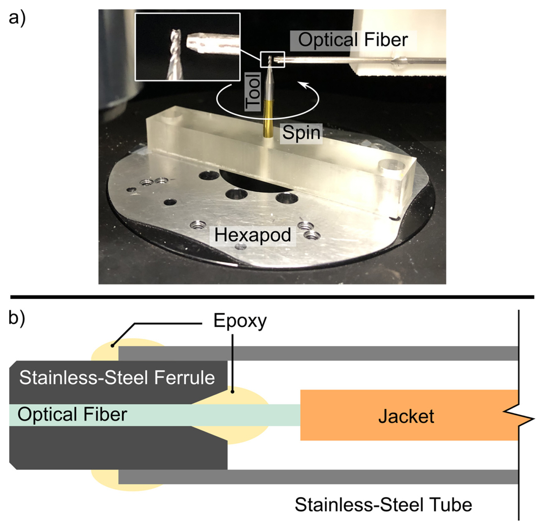
Fig. 2(a) shows the setup for tool profile 3D reconstruction The tool was held by the fixture with its axis pointing upward. The fixture was fixed on a 6-axis hexapod with a positioning accuracy of sub-micron level. The inset of Fig. 2(a) shows the detail of the tool and packaged optical fiber. Fig. 2(b) shows the structure of the packaged optical fiber. The bare fiber was fed through the center of a stainless-steel ferrule and was fixed at the end of the ferrule using epoxy. The stainless-steel ferrule was fixed at the end of a stainless-steel tube using epoxy. The packaged optical fiber was fixed on a fixture that will not move with the tool. The axis of the fiber was perpendicular to the axis of the tool. A gap was left between the end of the fiber and the surface of the tool. Therefore, an FPI was formed by the interface between the fiber and air and the surface of the tool. During measurement, the tool was rotated and moved upward after each rotation.
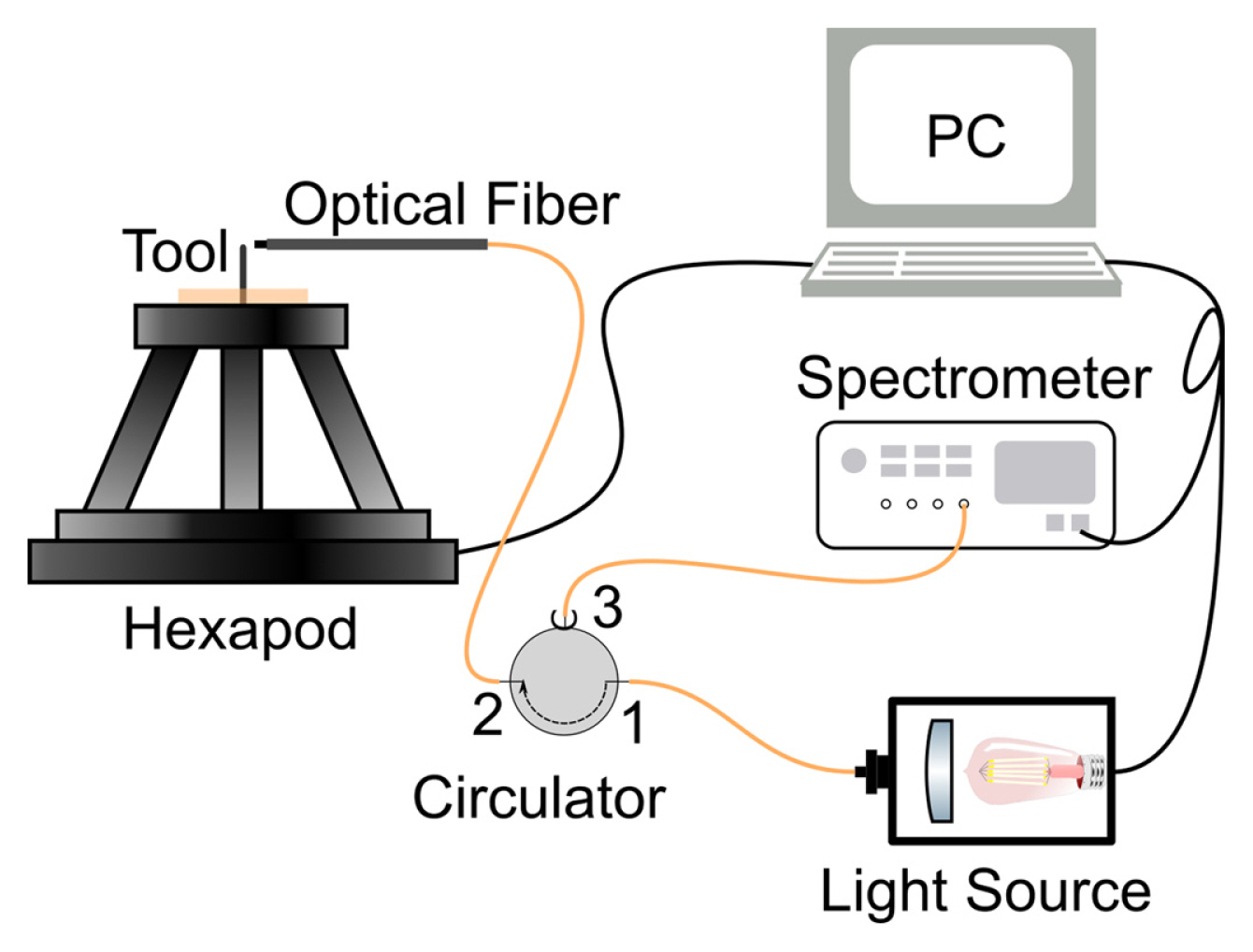
Fig. 3 shows the connection of the monitoring system. An optical circulator is a 3-port device that when light incident from port 1 will exit from port 2, and when incident from port 2 will exit from port 3. The incident light comes from the light source and then enters port 1. Then the output light from port 2 will propagate to the FPI formed by the fiber and the tool. The reflected light will propagate to the opposite direction along the fiber and enters port 2. The output light from port 3 will then enter the spectrometer. The light source, spectrometer, and hexapod were connected to the PC. The coordinates and the timestamps of the tool, as well as the corresponding spectra, were recorded by the PC. In this experiment, we analyzed the spectra and reconstructed the profile of the tool after the scan. The analyzing process can also be done during the scan process to realize a real-time profile reconstruction.
2.2.2 CNC Machine Straightness Error Monitoring
Straightness error is one of the innate geometrical errors from the machine tool that can largely influence the manufacturing precision [24–26]. However, straightness error can change while the load of the machine tool changes, and there is no portable online approach that can evaluate the straightness error instantly. Therefore, in this section, we refer to Ref. [25] and measure the straightness error of a milling machine tool with Sequential Two Point (STP) method using two optical fiber sensors. We have employed machine learning algorithm to accelerate the spectrum analyzing algorithm in order to realize an online straightness error measurement technique.
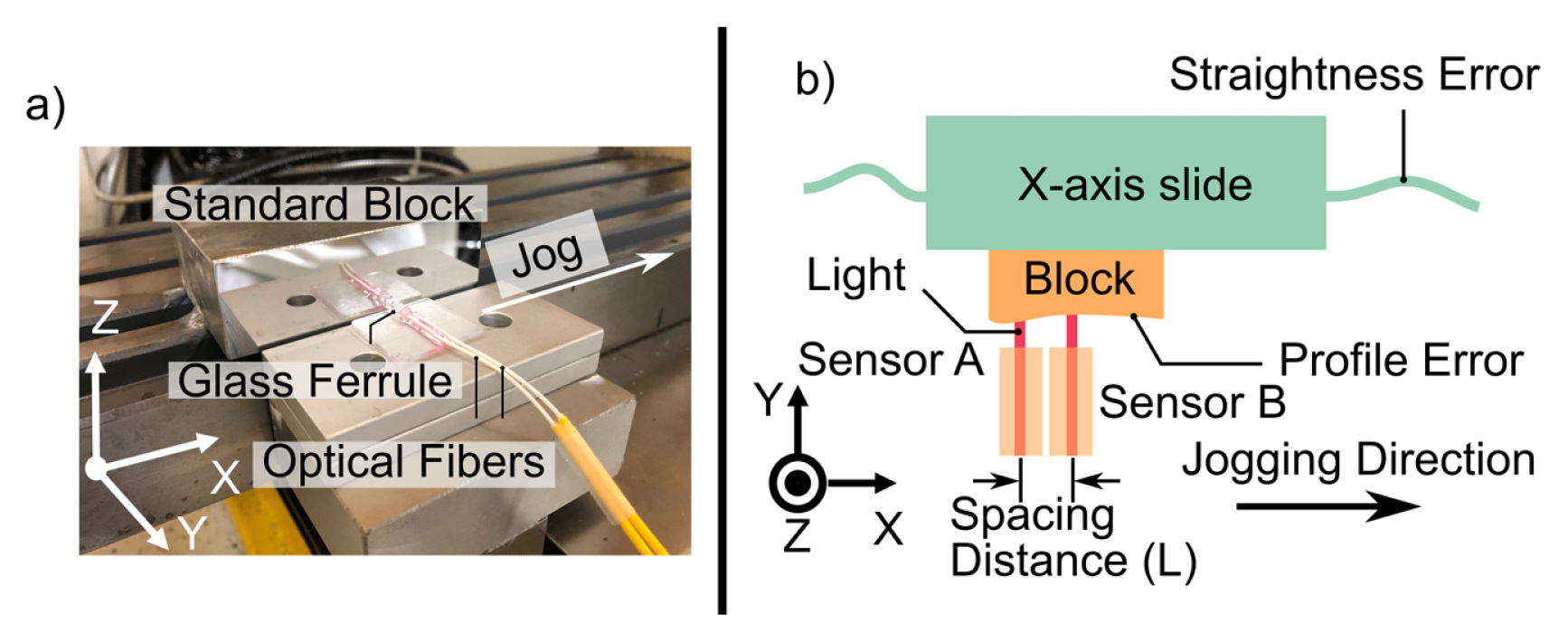
Fig. 4 illustrates the setup utilized for online straightness measurement. A commercially available CNC machine tool was employed to measure the straightness error of its X-axis guideway. Two optical fibers were installed on the machine tool's base using glass ferrules. These glass ferrules, together with the fibers, were affixed to the glass substrate using UV curable epoxy. The optical fibers were oriented perpendicular to the reference surface, facing in the positive direction of the Y-axis. A standard block has been mounted to the surface of the X-axis guideway and measured by these optical fiber sensors. While the standard block can move with the X-axis slide, the optical fibers remain fixed to the machine tool, enabling the measurement of the standard block’s profile.
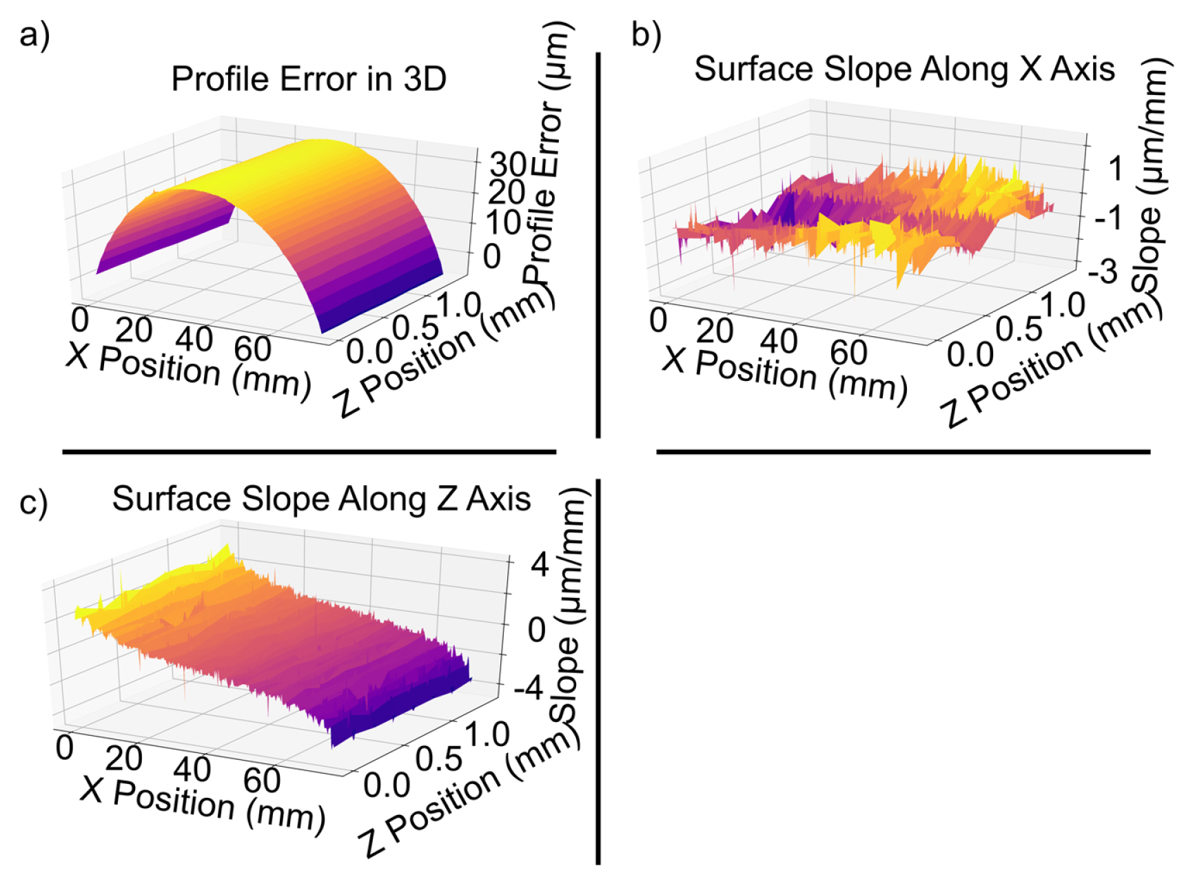
The standard block employed in this study is a low-cost 1-2-3 block, possessing a squareness of 0.003" per inch, a flatness of 0.002", and a parallelism of 0.002". According to Ref. [25], the polishing process has been carried out on an inexpensive polishing machine, and the profile of this polished surface has been measured by a precision Hexagon Coordinate Measurement Machine (CMM), shown in Fig. 5. The measured area is 1.4 × 75.0 mm large with the measurement spacing distance of 0.2 mm. The surface slope has been calculated based on this surface profile using the central difference approach. Ignoring the outliers, it appears that the surface slope along X axis is around -3 to 2 μm per mm, whereas that for Z axis is less than ±4 μm. This indicates that when deviation of the optical fibers along Y axis (or Z axis) is 1 mm, the measurement result from the optical fiber sensors contains -3 to 2 μm (or ±4 μm) error. Generally, the sum of the positioning error and the straightness error from the machine tool can be less than 100 μm along all directions. The assembly of the measurement setup has also been well adjusted to minimize the assembly error from X and Z. Therefore, the measurement error coming from the machine tool and the assembly of the setup can only contribute to sub-micron scale measurement error along Y axis, which guarantees an accurate measuring result. Two optical fibers were connected to the same interrogator using different channels to capture the wave spectrum of the reflected light. The spectrometer has a wavelength range between 1510 and 1590 nm. To have a better performance, the distance between the tip of the optical fiber and the polished surface of the standard block should be maintained between 200 to 500 μm. For this experiment, the initial gap was set to approximately 300 μm.
A PMAC motion controller (controller name, Delta Tau Data Systems Inc.) was used to control the position of X-axis, and it was connected to the same computer with the interrogator to coordinate the measurement and the machine tool’s movement. The optical fibers commence profiling the standard block from its right edge to the left edge while the X-axis slide moves in the positive direction from its relative zero coordinate, shown in Fig. 4. After every 100 μm jogging distance, the X-axis pauses for 5 seconds to allow the optical fiber sensors to obtain 10 measurement results at the same measurement point. The final measurement data was determined by selecting the value with the highest occurrence, effectively eliminating the influence of noise and machine tool vibrations. The analysis reveals that each measurement point has a minimum occurrence of more than 5, which guarantees the accuracy of the final measurement.
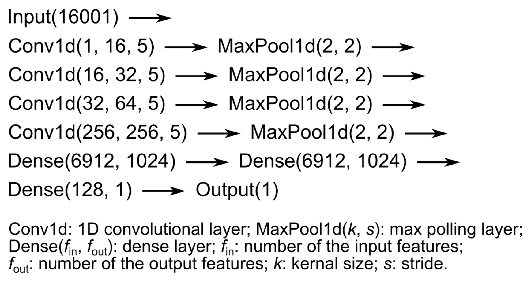
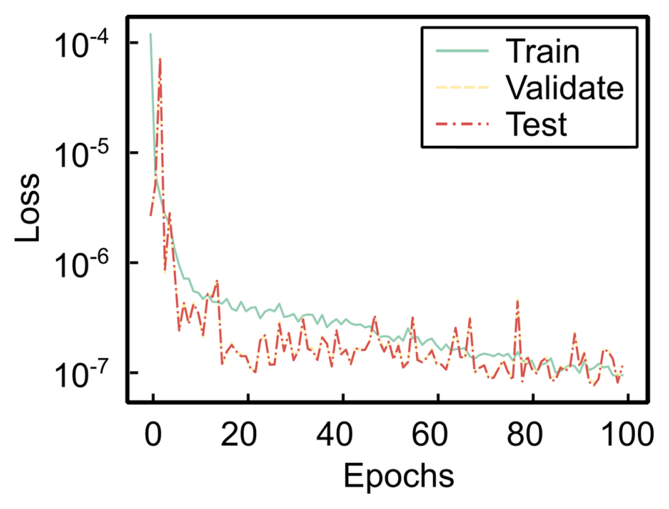
The overall measurement system is compactable and can be installed easily to any machine tool. In order to realize an online measurement system, deep learning has been employed to accelerate the spectrum analyzing process to predict the gap distance between the end of the optical fiber and the polished surface of the standard block. Since a distance of 67 mm has been measured and we conducted more than 10 measurements on a single measurement point, there can be around 6700 spectra generated from one optical fiber sensor (around 13+400 spectra for two optical fiber sensors for straightness error measurement). We conducted 14 straightness error measurement experiments and randomly selected 9 of them as the training dataset, 2 of them as the validation dataset, and 3 of them as the testing dataset (while the number of the spectra is 122339, 27116, and 54326 for training, validation, and testing dataset). The dataset input is a one-dimensional tensor which has 16001 features that depicts the spectrum between the power and the wavelength drawn directly from the interrogator. The label of the dataset is a scalar that is the normalized measured distance (that equals to
distance - 300 100
All the hyperparameters have been optimized using grid search. The first several layers of the neural network gradually deepen the channels of the input tensor and compress the tensor size while the last several layers have been designed to further extract important features from the input. 77 epochs have been applied for the neural network training according to the maximum validation accuracy. The final averaged prediction error is 0.3103 μm, 0.4886 μm, and 0.4782 μm for training, validating, and testing. The training/validating/testing loss is shown in Fig. 7.
3 Results and Discussion
3.1 Tool Profile 3D Reconstruction
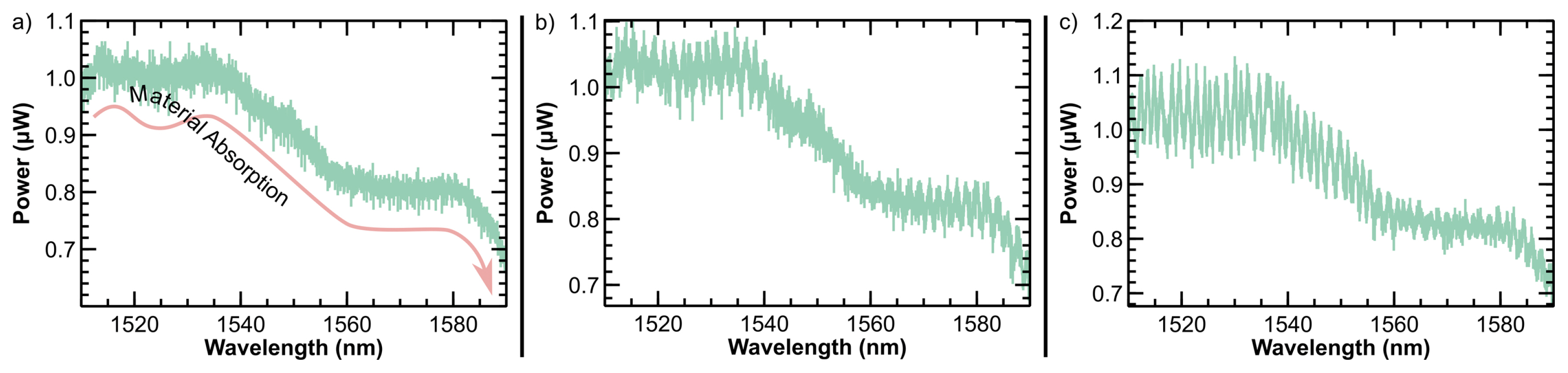
Due to the resonance in the FPI formed by the SMF-air interface and the air-tool interface, maximums and minimums can be observed in the reflected spectrum. However, an ideal FPI with two plane reflection surfaces requires a perfect alignment of the surfaces. However, the tool has a curved surface and therefore the two reflection surfaces cannot maintain paralleled all the time. Due to the diverge of the output light from the optical fiber, slight misalignment is still acceptable with a cost of lower contrast of the interference pattern. Fig. 8 shows different types of reflection spectra collected during this experiment. First, we can see a common trend of spectra shown as the translucent red curved arrow in Fig. 8(a). This is due to the absorption of the tool material which is determined by the molecular structure. Therefore, this absorption spectrum cannot provide us the distance information. Fig. 8(a) shows a poor spectrum due to a large misalignment between the fiber surface and the tool surface. This misalignment caused a low interference contrast that was completely covered by the noise. Therefore, it is difficult to get distance information from this spectrum. Fig. 8(b) shows a better spectrum compared with Fig. 8(a). As we can see, the interference pattern can be seen from this spectrum and therefore we can calculate the distance between the optical fiber and the tool surface. Fig. 8(c) shows a good spectrum of which the interference contrasts higher due to a small misalignment between the two reflection surfaces. Therefore, it is necessary to classify the quality of the reflection spectrum.
The character of a high-quality spectrum is the higher contrast of the interference pattern. Although the interference pattern is a chirped signal instead of a periodical function, Fourier Transform is still a good tool to classify the spectrum quality within a small range of wavelength (80 nm in this experiment). Since the fast Fourier transform (FFT) gives the spatial frequency of the spectrum, we can estimate the FSR by taking the reciprocal of its spatial frequency.
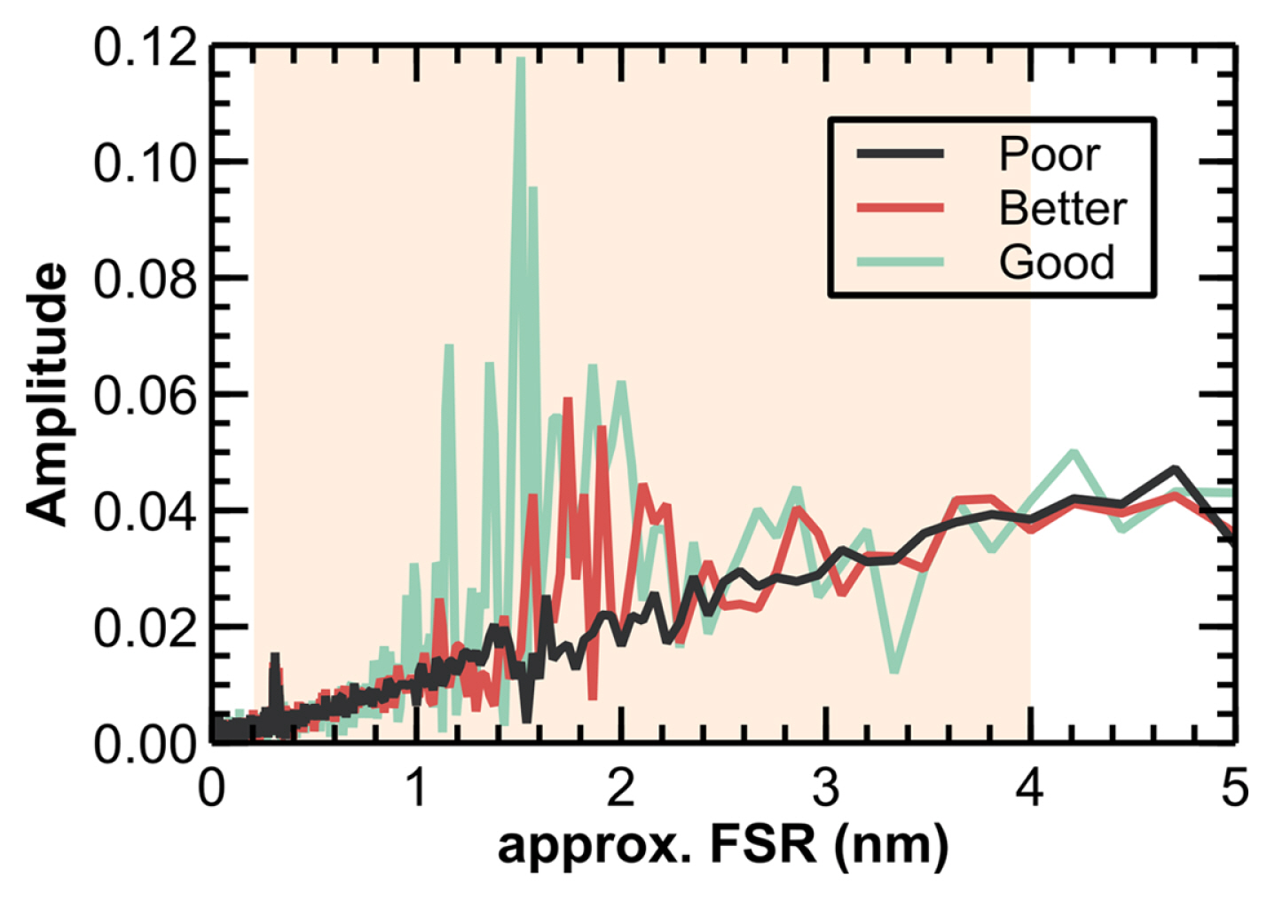
Fig. 9 shows the result given by FFT of the poor, better, and good spectra in Fig. 8. Before evaluating, we need to estimate the range of the FSR of the experimental spectrum using Eq. (4) since we know the range of the distance between the fiber and the tool. A quick estimation method in this experiment is take approximation of Eq. (5) as
since λm >> λFSR. Let, λm = 1550 nm, n = 1, and l ∈ [0, 3, 5] mm. Then we get λFSR ∈ [0, 2, 4] nm as shown in Fig. 9. For a poor spectrum, no significant peak can be seen within this range. And for better and good spectra, we can see significant peaks between 1 and 2 nm which agrees with their corresponding spectra in Fig. 8.
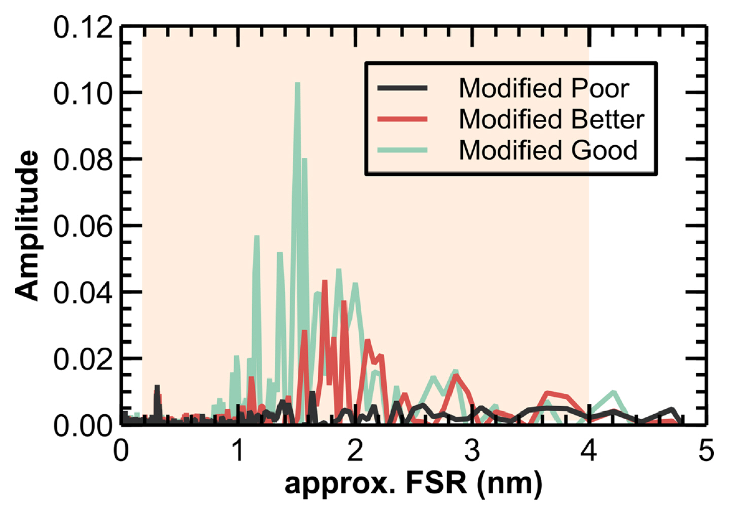
The method used in this experiment to quantitively evaluate the peak is fitting the FFT curve between 0 nm and 5 nm without the points between 0.2 nm 4 nm using a linear function. Then, subtract the fitting curve from the FFT curve. Fig. 10 shows the modified FFT of the three spectra. Then, we can simply find the maximum amplitude to determine the quality of the interference spectra. And we can use the wavelength corresponding to the maximum amplitude as λm.
To evaluate the resolution of the method based on Eq. (6), we need to know the resolution of the FFT. Ref. [27] gives the resolution of FFT in range [λ0, λ1] with sampling points N as:
Since the FSR is approximated as the reciprocal of the spatial frequency given by the FFT, the resolution depends on the spatial frequency (wavenumber) of the maximum amplitude of the FFT result. For spatial frequency at point fm and fm+1, the resolution of FSR is:
Therefore, the resolution depends on the spatial frequency with the maximum amplitude after FFT. Assume we have fm = 1/3 nm−1 for a spectrometer at rang 1510 to 1590 nm. Then the resolution is RFSR = 0.108 nm. Substitute to the Eq. (6) and use λm = 1550 nm, n = 1, and λFSR = 1/fm = 3 nm. We have the resolution of distance between the fiber and the target is Rod = 13.914 μm. To further improve the resolution, a manual process is given in Ref. [16]. The manual method has a theoretical resolution of 4.45 nm. To improve the efficiency of the manual method, a machine learning algorithm will be introduced in the following section. The measurement range of the FPI is determined by the quality of the signal. Using a spectrometer with a wavelength range from 1510 nm to 1590 nm, the distance between the fiber and the target between 100 μm and 4 mm can be monitored. In order to obtain a high-quality spectrum, the distance between the fiber and the target should be maintained between 200 and 500 μm.
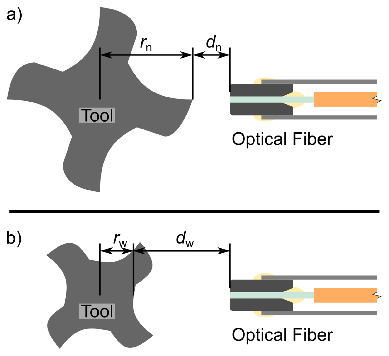
Now, since we know all the necessary parameters in Eq. (5), we can calculate the distance between the fiber and the tool. However, to recover the tool profile, we need some extra information about the tool. For a new tool, the outer diameter of the tool is usually provided by the vendor. The outer diameter can be used to calculate the distance between the measured point and the axis of the tool by knowing the distance between the measured point and the optical fiber. Fig. 11 shows the method to reconstruct the profile of the new and used tools. For new tools, we need to find the minimum distance between the optical fiber and the tool dn. With knowing the radius of the new tool rn, we can calculate the distance between the optical fiber and the axis of the tool as
Then, the distance between the measured points and the axis of the tool can be calculated as
where d is the distance between the optical fiber and the measured point. It should be noted that since we are monitoring the distance between the fiber and the tool, runout can be seen in the reconstructed profile. However, the existence can affect the accuracy of r, so it should be modified to compensate the radial and axial runout. To find the geometric center of the tool of each scan layer, we need the coordinates of at least three tips of the tool to determine the coordinates of the circle (xci, yci, zci) for the ith layer. With all the center coordinates, both the radial and axial runout can be calculated. Since we assumed rn was the distance between the tool axis and the tip, the calculate r was incorrect. Therefore, it should be recalculated after the runout effect is compensated. For tools with two tips, the process can be simplified since the center of the circle is at the center of the connection of the two tips.
For used tools, we assume that there is no wear on the points that are closest to the axis of the tool. Since the profile of the new tool has been constructed, we know the distance between the tool axis and the point that is closest to the axis, noted as rw. Finding the maximum distance between the fiber and the tool dw, then the distance between the optical fiber and the tool axis is now:
Therefore, the profile of the used tool can be reconstructed using the same method as Eq. (10).
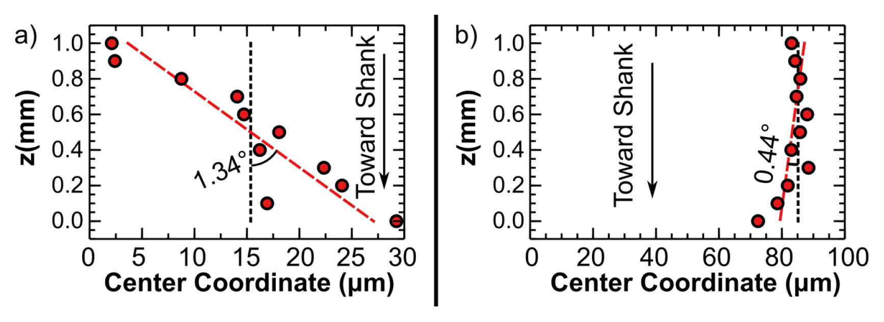
Milling tool runout error largely influences the chip thickness during the cutting which is one of the key factors that affects the milling quality [22,23]. This runout error can also be conducted by the 3D reconstruction of the milling tool. Before reconstructing the 3D profile, we need to calculate the runout of the tool first. As introduced before, we first assign a value between the rotation center and the tip of the tool (here we assign this value as 0.5 mm). With this value, we can reconstruct a 3D profile with an error of the distance between the monitored point and the axis of the tool. This error is caused by a proportional scale of the distance between the monitored point and the tool axis. Here we only need the coordinates of the tool axis, which is not affected by this scale, to calculate the runout. The distance between the monitored point and the tool axis should be corrected after compensating for both the radial and axial runout. Fig. 12 shows the shift of the reconstructed profile due to the effect of runout. Fig. 12(a) shows the coordinates of the tool center along the direction of the fiber axis, and Fig. 12(b) shows the coordinates of the tool center perpendicular to the fiber axis. The average coordinate along the fiber direction is s1 = 15.4 μm, and the angle between the tool axis and the vertical direction is α1 = 1.34°. For those perpendicular to the fiber axis, the values are s2 = 85.1 μm and α2 = 0.44°, respectively. Therefore, the radial runout is
s = s 1 2 + s 2 2 = 86.5 μ m a = arctan tan 2 α 1 + tan 2 α 2 = 1.41 °
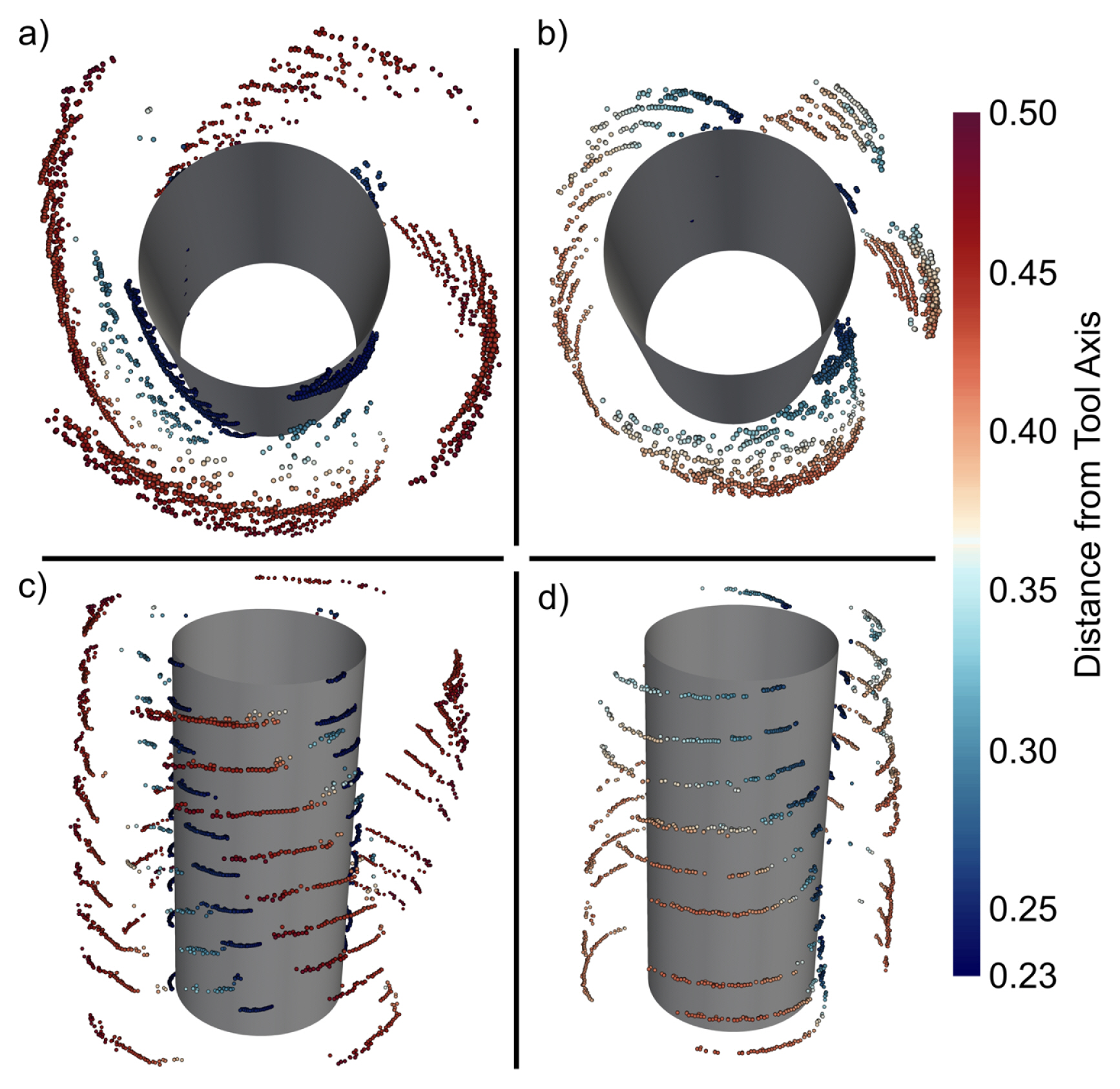
Fig. 13 shows the point cloud reconstruction of the tool profile, the color is the distance of the point from the tool axis. The scan step along tangential direction is 1°, and the scan step along the axis direction is 0.1 mm. Fig. 13(a) and Fig. 13(c) are the top and side of the reconstructed profile of a new tool, respectively. As we can see, the helix structure of the tool is reconstructed. The tips of the tool have a large distance from the axis compared with other points. However, because we throw away the low-quality spectra which are mostly the sampling points that are close to the tool axis, we get relatively less points close to the axis. Fig. 13(b) and Fig. 13(d) show the top view and the side view of a very worn tool. As we can see, the size of the tool along the radial direction is much smaller than that of the new tool. The blade was worn out therefore the outline of the tool has a rounded look compared with the new tool.
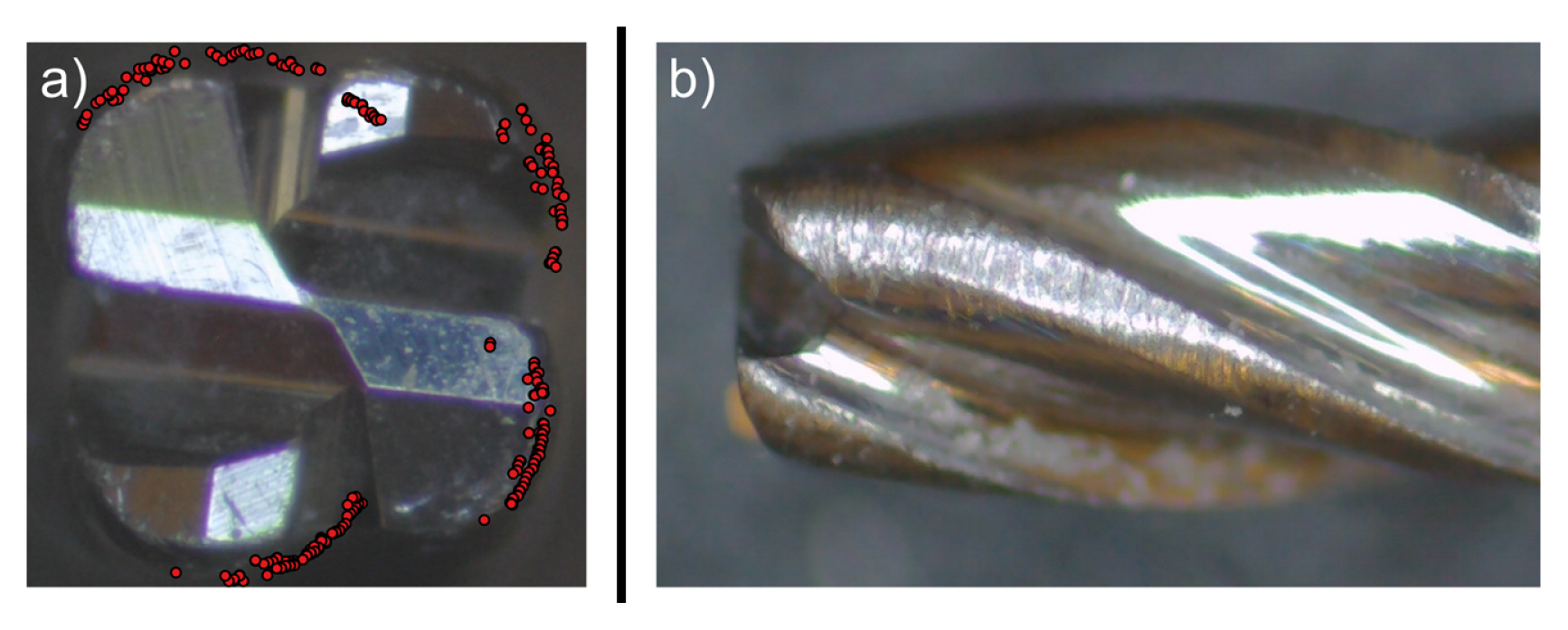
Fig. 14 shows the image of the used tool of top view and side view. Fig. 14(a) shows the top view of the tool and the matching with the point cloud. The points come from the first layer of the scan which is close to the top of the tool. As we can see, since the cutters were worn out, no sharp edges can be seen. Most points are located on the periphery of the tool, with a small number of points inside the periphery. There are two reasons for this difference: 1) the scanned points are located slightly lower than the top of the tool; 2) the points inside the periphery are on the flute of the tool due to this location difference. Fig. 14(b) shows the side view of the tool. We can see scratches on the side which indicate serious tool wear.
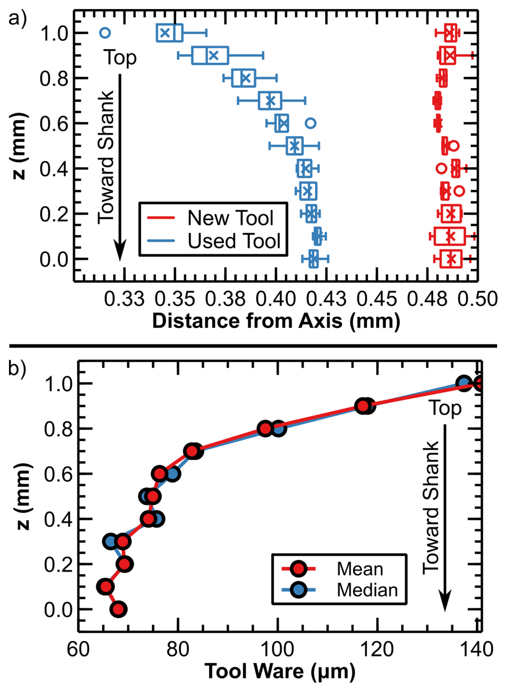
To quantitively evaluate the tool, we measured the distances from the axis to the 4 tips of the tool for each scanned layer. Fig. 15(a) shows the measurement of the measurements, the box plot (1.5IQR) of each layer is the statistics of the distances of the 4 tips. As we can see, for the new tool, the distances are close to the tool radius provided by the vendor (0.5 mm). The difference is because we calculate the radius based on the minimum distance between the tool surface and the fiber. According to the box plots, the measured value varies between 0.48 mm and 0.50 mm. One possible reason is that the sampled points may not be the tip of the tool exactly. Increasing the sampling number for each cycle can reduce this difference. For the used tool, we can see a curved shape of the profile. The distance between the measured point and the tool axis (radius hereinafter) on the top of the tool is the smallest. The radius increases towards the shank, which means less tool wear along this direction. Also, the radius of the four tips on the top of the tool shows a significant difference. This is because the nonuniform wear of the four cutters because of multiple reasons such as the runout of the tool. Towards the shank, the radius increases which indicates less tool wear. The tool wear can be calculated by taking the difference of radiuses between the new and the used tool as shown in Fig. 15(b). The tool wears are calculated based on both the mean and the median since there are some differences between them due to the outliers. As we can see, the tool wears calculated by mean and median have a similar tendency. At the top of the tool, a maximum tool wear of about 140 μm can be observed. Moving toward the shank, the tool wear reduces to about 68 μm.
3.2 CNC Machine Straightness Error Monitoring
We have employed Sequential-Two-Point (STP) method to separate the straightness error of the machine tool guideway and the profile error of the standard block. We use two optical fibers as displacement sensors, shown in Fig. 4(b), whose spacing distance is L. The raw sensor outputs, PA(x) and PB(x) from the displacement sensor A and B respectively, can be represented by:
where f(x) is the profile error from the standard block, and ey(x) is the straightness error of the X-axis guideway along Y-axis direction. Here, xn = n · L, and n = 0, 1, 2, 3, ..., N which illustrates the measurement position. The output difference between these two sensors can eliminate the straightness error term and provides the increment of the profile error. Therefore, the equation for the separated profile error f (x) and the straightness error e(x) can be expressed by:
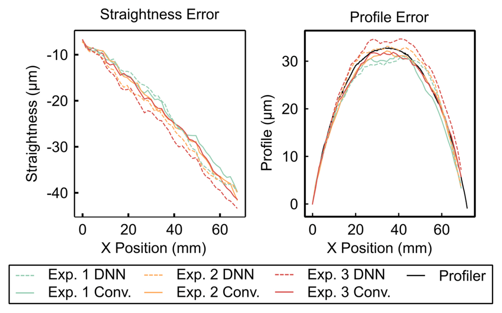
Using Eq. (12), we have conducted error separation technique on three experiments (that are also the selected testing dataset). The separated straightness error and the profile error using both the conventional spectrum analysis method are shown in Fig. 16. The spectra from two optical fiber sensors have been processed by both the conventional method (“Conv.” in Fig. 16) and the deep learning method (“DNN” in Fig. 16). The calculated profile error has been compared with the measurement result (“Profiler” in Fig. 16) from a CMM (Model name, Company name). It can be seen that the calculated profile error is very close to the CMM measurement result. The standard block has around 30 μm profile error over 67 mm range, and the straightness error of the machine tool guideway is around 40 μm. Though the deep learning method contributes to a larger prediction error, the overall accuracy can still be maintained. Further, the deep learning approach is able to process more than 6700 spectra from one optical fiber sensor in batch within 50.727 s, which guarantees the online measurement capability.
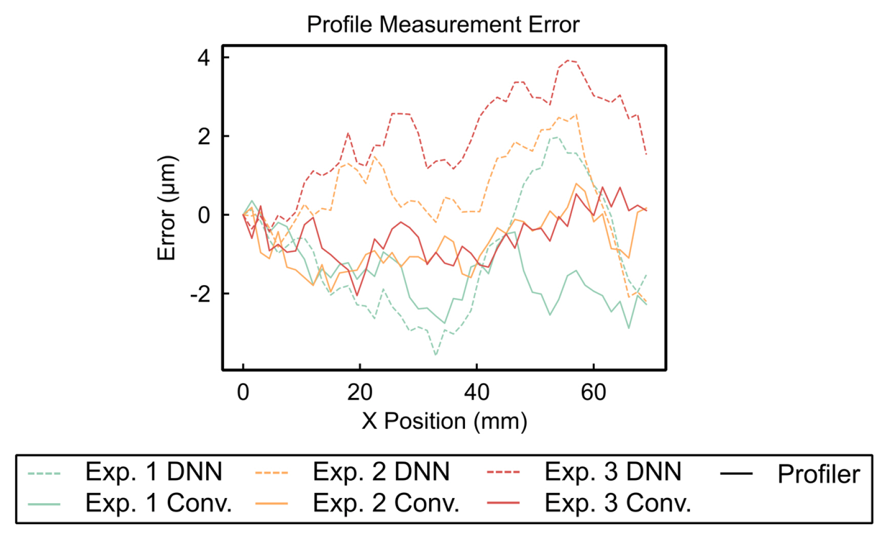
Also, we calculated the difference between the separated profile error and the measurement result from the CMM, shown in Fig. 17. It can be seen that, with the conventional method, the first two experiments have a measurement error of around 2 μm, while the error from the third experiment is a bit larger, which reaches around 3 μm. The results based on the deep learning method are larger since the average prediction error of the deep learning method can be around 0.5 μm. This prediction error from each measurement point can accumulate according to the summation process in Eq. (2). However, the largest measurement error based on the deep learning method is under 4 μm, which is still acceptable considering the overall 30 μm profile error. The deep learning method provides a compromised prediction result with a much faster speed, which broadens the application field of this portable straightness error technique. The straightness error measurement can be both cost efficient and time efficient.
4. Conclusion
In this research, we introduced a method to use optical fiber Fabry-Pérot interferometer (FPI) as distance sensor and its application in smart manufacturing. The measuring system includes a broadband light source, a spectrometer, an optical circulator, and the supporting spectrum analyzing algorithm. The Fast Fourier Transform (FFT) method was used to calculate the distance between the optical fiber and the surface of the target. To improve the speed of the spectrum analyzing process, neural network models were built to find out the distance between the fiber and the target.
First, optical fiber FPI was used to measure the distance between a fixed fiber and a rotating tool. With the rotation of the tool along its axis, the distance between the fiber and the surface of the tool was measured. With a selection of effective reflection spectra, the 3D profile of the tool can be reconstructed. By reconstructing the profile of a new tool, the runout of the spindle was calculated by finding out the deviation of the center of the reconstructed 3D profile from the origin. The tool wear can also be found by comparing the reconstructed profile of the new and the used tools. The analyzing method was introduced, which is robust for even noisy spectrum. However, the analyzing method is slow since large amounts of calculations are needed. To improve the analyzing speed, machine learning models were trained to find out the distance between the fiber and the target surface. Both CNN model and DNN model were developed and the difference between these models were compared. It was found that the DNN model has a faster speed compared with the CNN model. We applied the machine learning algorithm to measure the straightness error of a CNC machine. The result shows that the machine learning algorithm has an error of under 4 μm compared with the measurement given by a Hexagon Coordinate Measurement Machine. This difference can come from both the measurement of the optical fiber sensors and the Coordinate Measurement Machine. Moreover, the difference of the measurement location on the standard block can also introduce differences between the measurements.
Compared with mechanical methods, the proposed method is a noncontact method that has a high measurement precision. Compared with the commercially available interferometers, the proposed method is based on the wavelength of the interference spectrum instead of intensity. Therefore, the proposed method is more robust to environmental fluctuations which can cause a change of absorption in the air of the detection light. Moreover, the sensitive element of the proposed method is compact and therefore it is suitable for monitoring in a limited space.


 PDF Links
 PubReader
 Full text via DOI
 Download Citation
  CrossRef TDM


