Bayesian Hyper-parameter Optimization in One-dimensional Convolutional Autoencoder for Monitoring Bearing Health Status

Sungeu Chae; Suk Joo Bae

doi:10.57062/ijpem-st.2023.0115

Int. J. Precis. Eng. Manuf.-Smart Tech. > Volume 2(1); 2024 > Article

Chae and Bae: Bayesian Hyper-parameter Optimization in One-dimensional Convolutional Autoencoder for Monitoring Bearing Health Status

Regular Paper

International Journal of Precision Engineering and Manufacturing-Smart Technology 2024;2(1):15-22.

Published online: January 5, 2024

DOI: https://doi.org/10.57062/ijpem-st.2023.0115

Bayesian Hyper-parameter Optimization in One-dimensional Convolutional Autoencoder for Monitoring Bearing Health Status

Sungeu Chae¹ · Suk Joo Bae¹

¹Department of Industrial Engineering, Hanyang University, Seoul, Republic of Korea

Suk Joo Bae, sjbae@hanyang.ac.kr

Received November 29, 2023 Revised December 20, 2023 Accepted December 20, 2023

Abstract

This study introduces a framework that integrates hyperparameter optimization techniques for feature representation and abnormality detection in machine health diagnostics. The framework leverages one-dimensional convolutional autoencoders (1D-CAEs) and multilayer perceptron (MLP) as the key components. We propose a systematic approach that begins with the development of the 1D-CAE model to encode characteristics into a latent vector. Subsequently, we employ an MLP to effectively detect and identify abnormalities within the encoded data. Our study presents a novel contribution by integrating an adjusted hybrid stopping criterion into the Bayesian optimization framework to improve the efficiency and robustness of anomaly detection. The accuracy and training time of these approaches were examined and evaluated using the bearing degradation data under real-life scenarios. The findings of our study provide strong evidence that the utilization of the Bayesian optimization method, along with the suggested stopping criterion, surpasses conventional tuning techniques in both training time and accuracy. This achievement sets a novel standard for optimizing hyperparameters in the prognostics and health management field. The superiority observed in our study extends beyond the fidelity of the derived models, encompassing the accelerated identification of ideal hyperparameters and holding practical value for real-world applications for early detection of abnormality.

Keywords: Latent feature representation · Adjusted hybrid stopping criterion · Predictive maintenance · Hyper-parameter tuning strategies

1 Introduction

For health diagnostics of machines or equipment, the accuracy of feature representation and the effectiveness of abnormality detection are crucial factors. This study examines these factors via the capabilities of Bayesian optimization for hyper-parameter tuning in 1D-CAE for encoding latent vectors and MLP for subsequent identification of anomalies. In acknowledging the advancements made by Längkvist et al. [1] and other studies [2–6] in the application of autoencoders and their variations, we aim to extend this investigation by explicitly optimizing the hyper-parameters in CAE architecture for enhancing the analysis of time-series signal data. CAE structure, which was evidenced by Masci et al. [7] and Du et al. [8] in image datasets and adapted by Liu et al. [9] for noisy signal data, showed versatile achievements in the field of biomedical imaging and machine health diagnostics, where these models have demonstrated commendable performance in classification of features of interest.

An integral aspect of our research is the systematic fine-tuning of the hyper-parameters of the Adam optimizer, which is crucial for achieving optimal performance of the 1D-CAE model through a well-planned gradient descent approach. The Adam optimizer has gained significant prominence in the field of deep learning due to its efficacy in managing sparse gradients and its capacity to adapt to big datasets. However, it should be noted that predetermined hyper-parameters of the Adam optimization algorithm, while generally reliable, may not be globally optimal in every situation. In this discourse, we examine Grid search, Random search, and particularly, Bayesian hyper-parameter optimization methods that have been extensively examined and contrasted in research works. Bergstra and Bengio [10] expressed their preference on Random search method as a superior approach compared to Grid search. However, Jones et al. [11] has emphasized the potential benefits of Bayesian optimization. Our research builds upon the aforementioned findings by proposing a modified form of the adjusted hybrid stopping criterion that boosts the effectiveness of optimization, as previously suggested by Lorenz et al. [12].

This study introduces a novel framework to overcome the limitations of conventional hyper-parameter optimization methods in anomaly detection. The proposed approach integrates a modified form of the adjusted hybrid stopping criteria-based Bayesian hyper-parameter optimization technique with 1D-CAE for feature representation and anomaly detection. The objective of this strategy is to achieve a high level of accuracy in detecting abnormalities, while also minimizing the amount of computational time required for training. The primary contributions of this study are:

1. Automate feature extraction for time series signal data, eliminating the arduous task of manual feature engineering and minimizing information loss.
2. Enhance the representation of signal data characteristics by robustly learning features, thereby diminishing noises and variations that are typical in machine health diagnostics.
3. Utilize Bayesian optimization to refine generalization capabilities of the proposed framework, ensuring reliable model performance across different machine states and scenarios.

The subsequent portions of this paper will be presented in the following manner: Section 2 explores the complexities of CAE architecture, Bayesian optimization, and adjusted hybrid stopping criteria. Section 3 presents experimental validations of the proposed framework and compares the performance of the proposed framework with standard approaches. Section 4 synthesizes our key findings and suggests potential directions for future research in the domain of machine health diagnostics.

2 Background Theory

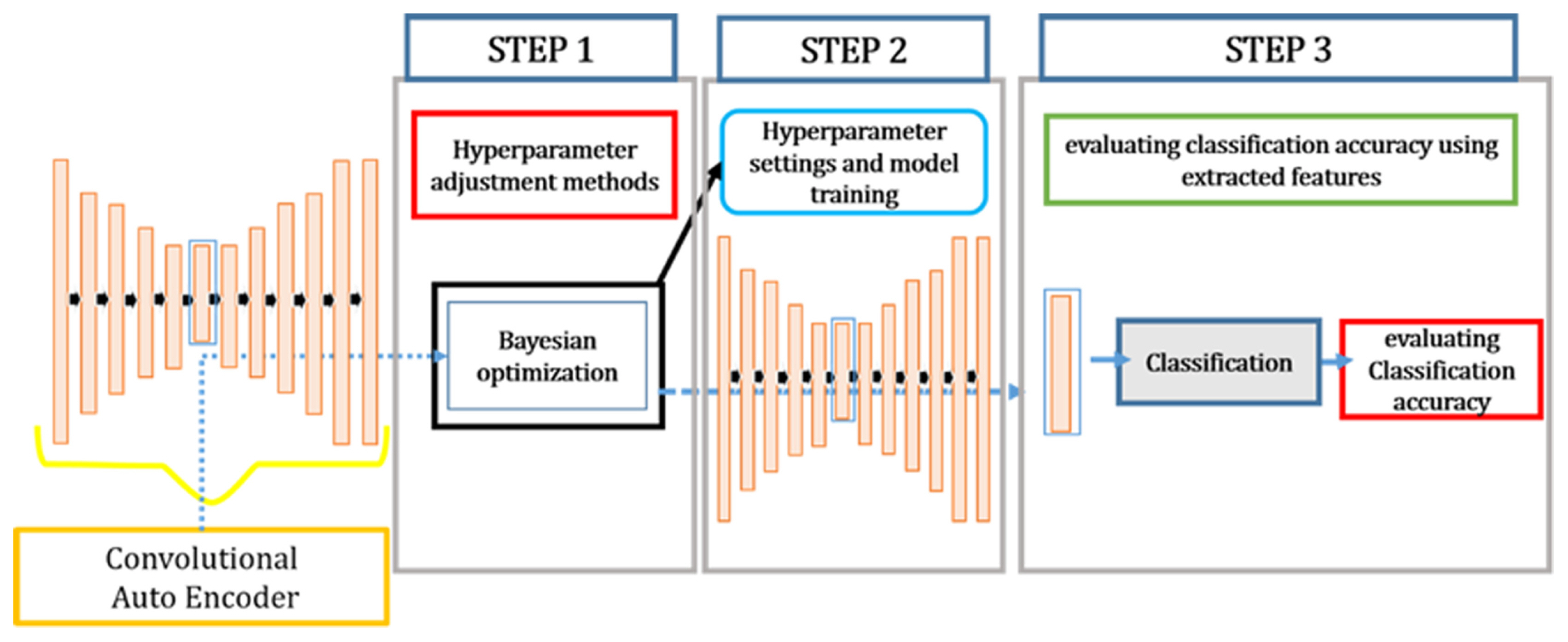
The present investigation incorporates the procedural framework outlined in Figure 1. The 1D-CAE architecture as a model for unsupervised learning is employed to extract inherent properties of the time-series signal data. The performance assessment of the proposed model is performed by introducing a loss function. It has been commonly assumed that a reduction in the loss function is an indicator of enhanced efficiency in both compression and feature extraction inside the hidden layer. Therefore, in the preliminary phase, the Bayesian optimization as a method for automatic adjustment of hyper-parameters is implemented to minimize the loss function of the proposed model. In the subsequent phase, the hyper-parameter values that result in the lowest loss function during the initial step is used as an input to this model such that the compressed layer contains condensed characteristics of the data. During the third step, the hidden layer is incorporated as an input parameter, then the multilayer perceptron classifier is employed to evaluate the accuracy of anomaly detection in classification.

2.1 1D-convolutional Autoencoder

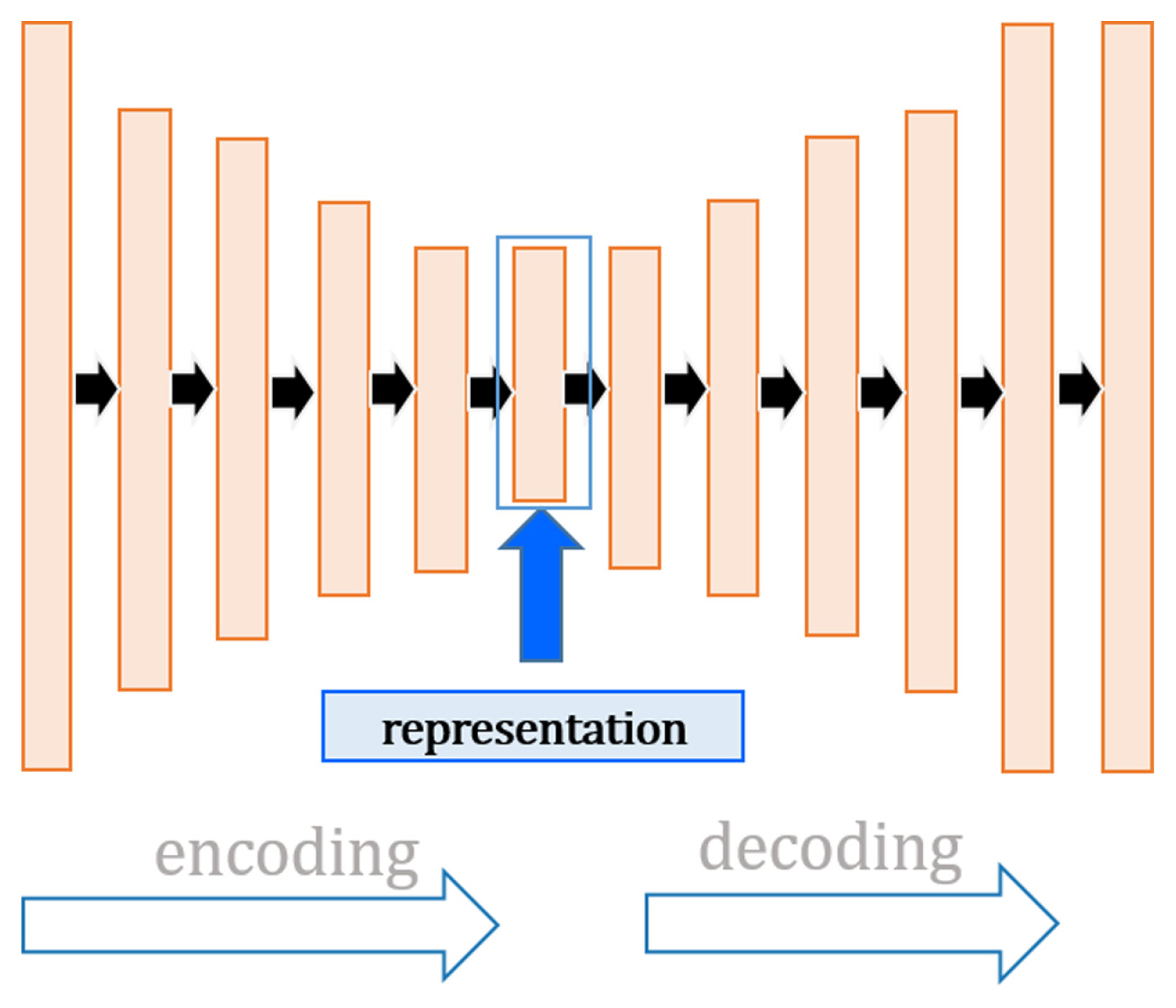
In the referenced literature [13], autoencoders were elucidated as sophisticated neural architectures engineered to distill pivotal characteristics from high-dimensional data by leveraging two integral components: an encoder and a decoder. These devices for dimensionality reduction operate on the principle of creating a compressed representation of the input vectors x_i, which are then regenerated as x̂_i in the output to foster a harmony of dimensions between these two layers. This is instrumental for the autoencoder to learn and reconstruct the input data effectively.

Specific to our research, the 1D-CAE is adopted as a framework for feature representation, wherein autoencoders are organized in a convolutional schema. This structure is pivotal as it allows to extract salient features from the input data independent of any label assignments, hence emphasizing its unsupervised learning capability.

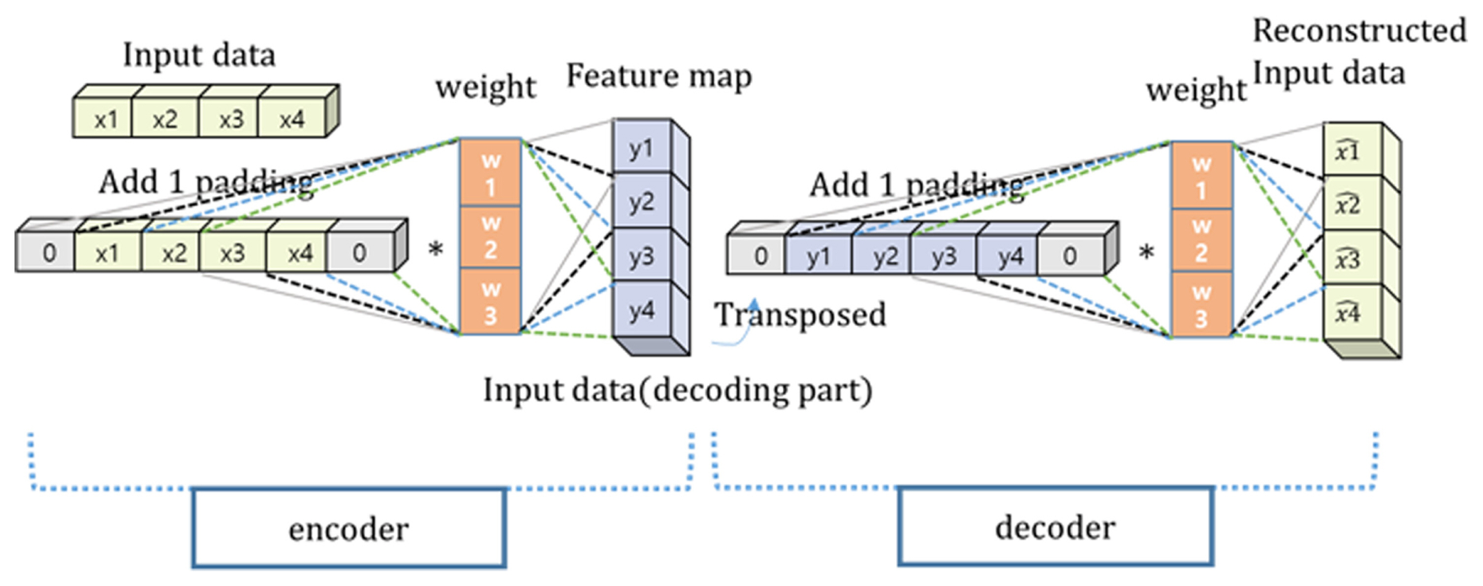
The 1D-CAE mirrors the structural essence of a classic autoencoder but distinguishes itself through the employment of shared weights across its convolutional layers. These layers utilize one-dimensional convolutional kernels to parse through the input vectors, generating localized feature maps. Each map is then transformed via a non-linear activation function, echoing the methodologies used in one-dimensional convolutional neural networks (1D-CNNs), a process visually explicated in Figure 2.

Subsequent to convolution, derived feature map is subject to a subsampling procedure within a dedicated layer, effectuating a reduction in the feature dimensionality. Here, N input maps culminate in N refined output features, with the downsampling dynamics described by the equation:

(3)

xjl=f(βjl·down(xjl-1)+bjl), j=1,2,…,N,

where down(·) is the subsampling operation, and the terms β and b correspond to multiplicative and additive parameters, respectively. The subsampling function, down(·), amalgamates multiple (n × 1) dimensional input feature maps into a compressed output of reduced dimensionality 1/n.

The encoder phase culminates with the application of convolution and downsampling on the input vectors. Contrastingly, the decoder phase inverses this methodology as it endeavors to reconstruct the original input data, as depicted in Figure 3 . Both phases of the 1D-CAE—encoding and decoding—harness convolutional operations to refine high-level feature abstractions from the input data. The encoder selectively filters the data through the application of one-dimensional convolutional kernels and a Tanh activation function to extricate relevant features, while the decoder reconstructs initial input data from these features, navigating through and diminishing the interference of process noises.

An issue commonly raised by deep neural architectures such as autoencoders is the vanishing gradient problem, as documented in studies [14,15]. A contemporary solution involves incorporating residual connections within the autoencoder framework, leading to the inception of the residual autoencoder (RAE) or the ResNet AE [16]. Our investigation delves into the synergy of the ResNet design with the 1D-CAE model to bolster its learning efficiency through the integration of residual blocks. These blocks are efficient in alleviating the vanishing gradient quandary that is frequently encountered in deep learning networks. This enhancement empowers the 1D-CAE to proficiently capture and represent complex feature hierarchies, thereby augmenting its reconstruction fidelity. The mathematical representation of a residual block within the ResNet paradigm is depicted as:

(4)

y=F(x,{Wi})+x

wherein x and y are the respective input and output of the residual block, F symbolizes the residual function to be ascertained, and [W_i] is the ensemble of weights within the block. This residual learning strategy enables networks to be trained by reforming the layers to learn residual functions concerning the inputs of the layers, rather than learning functions without any reference.

Finally, the loss function governing the performance of the 1D-CAE is articulated as follows:

(5)

Loss=avg|X-X˜|2

where X and X̃ denote the input and the output of the encoder, respectively. The gradient descent algorithm is harnessed to minimize the reconstruction error. In this investigation, we employ the Adaptive Moment Estimation (ADAM) optimization algorithm proposed by Kingma and Ba [17] to efficiently drive the minimization of the reconstruction discrepancy.

2.2 Bayesian Optimization

In the scope of this investigation, we optimize the hyper-parameters of the proposed neural architecture by employing Bayesian optimization, which accelerates the convergence towards the most effective values of the objective function that is exemplified by the sum of squared errors (SSE). Bayesian optimization is a potent technique for the optimization of computationally demanding functions, drawing upon the principles of Bayes’ theorem of conditional probability, expressed as:

(6)

p(w∣D)=p(D∣w)p(w)p(D),

Here, p(w) denotes the prior probability of an unobserved variable w,p(D|w) is the likelihood, and p(w|D) symbolizes the posterior probability.

The Bayesian optimization methodology refines its search for optimal hyper-parameter values by utilizing information gleaned from previous iterations through an acquisition function. This function is instrumental in identifying the subsequent observation that is most likely to yield a maximum in the objective function. Noteworthy acquisition functions include the probability of improvement (PI), expected improvement (EI), and upper confidence bound (UCB). The goal of the Bayesian optimization in this work is to find the hyper-parameters minimizing the objective function within the evaluated search space. The Gaussian process regression (GPR) serves as a surrogate model to probabilistically forecast the objective function, extending the multivariate Gaussian distribution to an infinite-dimensional stochastic process where any finite dimensional marginalization remains Gaussian as

(7)

f(x)≈GP(m(x),k(x,x′)),

where m(·) and k(·,·) represent the mean function and the covariance function in GPR, respectively. A commonly utilized covariance function is the squared exponential, which is defined as

(8)

k(xi,xj)=exp(-12|xi-xj|2),

By applying both the acquisition function and the GPR surrogate model to the loss function, Bayesian optimization outperforms the methods such as random sampling in efficiency. The algorithm underpinning the proposed Bayesian optimization alternates between updating the posterior distribution and maximizing the acquisition function as detailed below, where D1:t-1={xn,yn}n=1t-1 comprises the training dataset with (t – 1) instances for the surrogate model f.

Regarding termination criteria for Bayesian optimization, Golovin et al. [18] employed the median stopping rule, which compares the average of updated function values with the historical function values. Termination occurs when the current value is substantially lower than the historical average, although this requires a predefined threshold, which adds the complexity due to an additional hyper-parameter.

In contrast, our research adopts the adjusted hybrid stopping criterion to enhance the method initially proposed by Lorenz et al. [12]. The original hybrid criterion used EI during the Bayesian optimization process, along with PI for interpretability. PI specifically calculates the highest probability of an improved objective function value in subsequent samples, akin to a Z-test. The adjusted hybrid stopping criterion refines this by setting a significance level α for the hypothesis testing framework: H₀:μ(λ) > f(λ⁺) versus H₁:μ(λ) > f (λ⁺), where the p-value is derived from γ(λ). Here, γ(λ) represents the degree of improvement and PI(λ) = Φ(γ(λ)) represents the probability of improvement, where γ(λ) is expressed. as

(9)

γ(λ)=μ(λ)-f(λ+)+ɛσ(λ)

where λ⁺ is the set of hyper-parameters that maximizes the objective function so far and ɛ is the minimum amount of improvement required for the best function value observed. In the adjusted hybrid stopping criteria, the optimization process halts when the p-value falls below significance level α, suggesting a significant likelihood of the new sample exceeding the current best observation.

The following table compares the original hybrid stopping criteria with the proposed adjusted hybrid stopping criteria.

3 Results and Discussion

This section provides experimental setups to collect comprehensive comparative data of hyper-parameter optimization methods and discussions on the findings from the results. The data are collected under four test scenarios, namely Grid search, Random search, Bayesian hyper-parameter optimization and the baseline scenario. Based on the comparative analyses, we aim to develop and validate the proposed framework for accurately detecting anomaly using shorter training time, which contributes to faster on-line detection of failures.

3.1 Experimental Setup

Experimental design encompasses three phases, aimed at collecting data on the efficacy of various hyper-parameter optimization strategies for our predictive model. The initial phase involves an exhaustive exploration for the optimal set of hyper-parameters that minimize the loss function within 1D-CAE architecture. The parameters in question include the learning rate and regularization terms for the Adam optimizer. These parameters were subject to both Grid search and Random search techniques. For the Grid search, parameters were systematically varied across five evenly spaced values within the pre-established range as shown in Table 2, leading to numerous potential parameter combinations. In contrast, Random search and Bayesian optimization were conducted within the ranges specified in Table 3, based on preliminary values deemed as effective in the seminal work of Kingma and Ba [17]. The epoch and batch size were held constant across all of the models at 50 and 128, respectively, to ensure consistency outside the optimization process.

The second phase entailed the application of the best hyper-parameter set ascertained from Grid search, Random search, and Bayesian optimization, utilizing an adjusted hybrid stopping criterion with an EI threshold. Additionally, baseline parameters, α = 0.001, β₁ = 0.9, and β₂ = 0.999, as defined by default in Kingma and Ba [17], were tested for comparative purposes. In the third phase, latent features from phase two were served as the input for a multilayer perceptron neural network classifier to assess its ability to accurately classify bearing anomalies post the 710th cycle, as illustrated in the research by Kim et al. [19]. The experiments were facilitated by a computing environment with an Intel Core i7-8750H CPU, 16GB RAM, and an NVIDIA GeForce GTX 1070 GPU.

3.2 Data Description

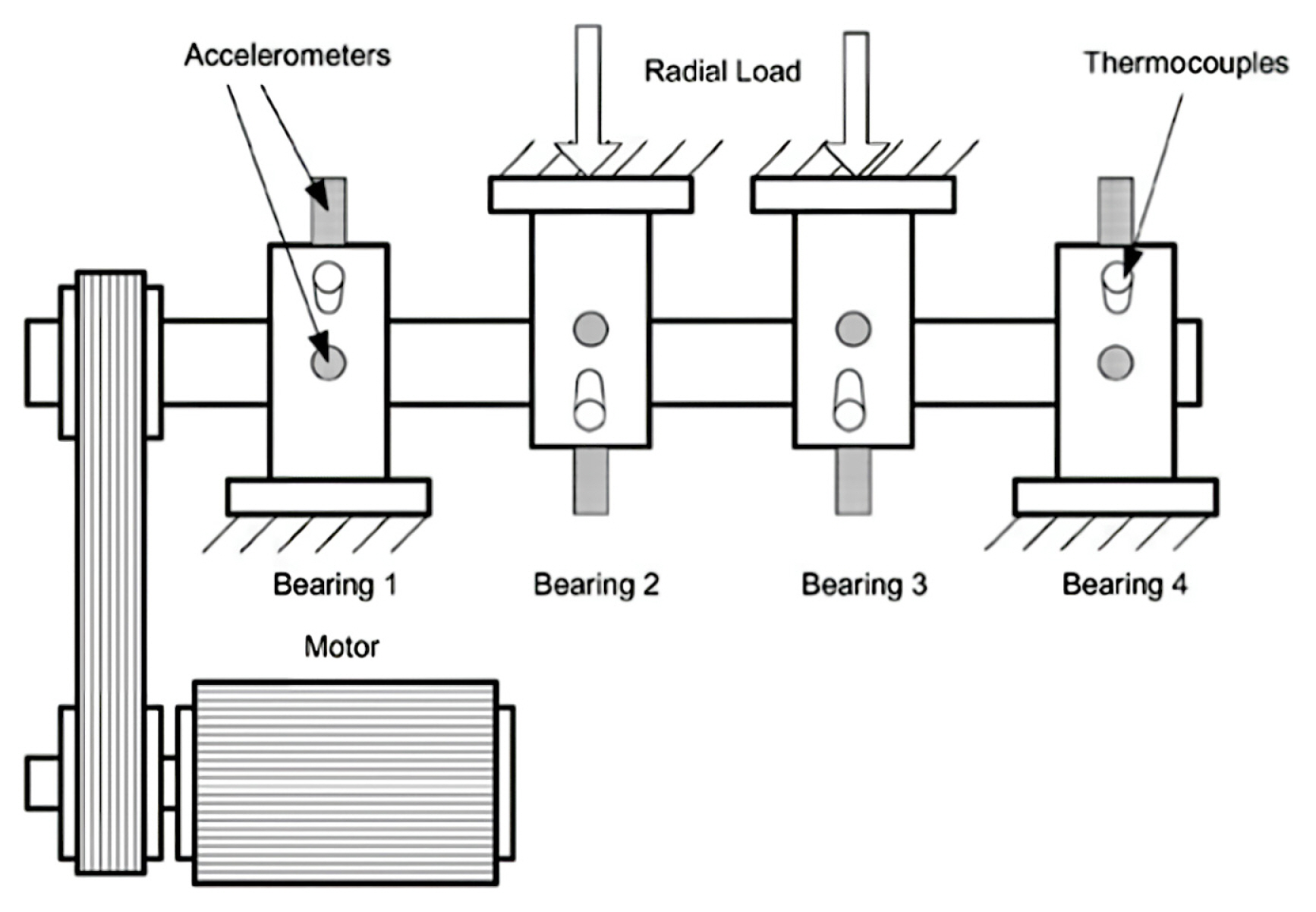
The datasets used in the experiment to provide a comparison and enhance the validation are sourced from NASA IMS. The IMS file has three distinct testing datasets, whereby each dataset includes operational data pertaining to the monitoring of four bearings. The initial dataset comprises monitoring outcomes for each bearing in both the horizontal and vertical orientations, while the second and third datasets solely encompass the monitoring outcomes for the bearing in a single direction. During the monitoring procedure, the bearings exhibit a consistent rotational speed of 2000 revolutions per minute, which is facilitated by an alternating current motor. Data are taken at regular intervals of 10 minutes, with a sampling frequency of 20.48 kilohertz [20]. The datasets contain the signal recordings spanning from initial functioning of the bearing to its eventual breakdown. The present study examines the second dataset, which encompasses monitoring data related to the functioning of four distinct bearings. Every individual bearing is equipped with a single sensor that captures the vibration data of 20,480 specific points during each recording instance.

3.3 Hyper-parameter Optimization for Adjusted Hybrid Stopping Criteria

The first experiment primarily focuses on the optimization of hyper-parameters for a stopping criteria of Bayesian hyper-parameter optimization for 1D-CAE framework. The main emphasis was placed on determining the optimal level of improvement, denoted as ɛ, within the context of adjusted hybrid stopping criteria using the objective function value, loss from 1D-CAE as a criterion. Both the original and adjusted hybrid stopping criteria were evaluated with a significance level set at α = 0.01 and baseline hyper-parameters for 1D-CAE. For the original hybrid stopping criteria, the experiment terminated with the most notableg termination at ɛ = 1.0, yielding an objective function value of 0.0138. In contrast, the adjusted criteria demonstrated enhanced performance, concluding the experiment at a superior objective function value of 0.0121 when set at the same ɛ level, highlighting the effectiveness of the adjusted method in refining our 1D-CAE model.

3.4 Performance Evaluation

The second experiment’s results are elucidated in Table 5, which contrasts the loss values and computation times across the three hyper-parameter optimization approaches. The Grid search identified a minimum loss value after an extensive 159 minutes, whereas the Random search achieved its best result within just over 11 minutes. Significantly, Bayesian optimization surpassed both, attaining its minimum loss in a mere 3 minutes and 16 seconds, indicating a substantial reduction in computational demand over 53 times faster than Grid search. It is crucial to recognize the inherent variability in the Random search’s time efficiency, dependent on both data characteristics and model structure.

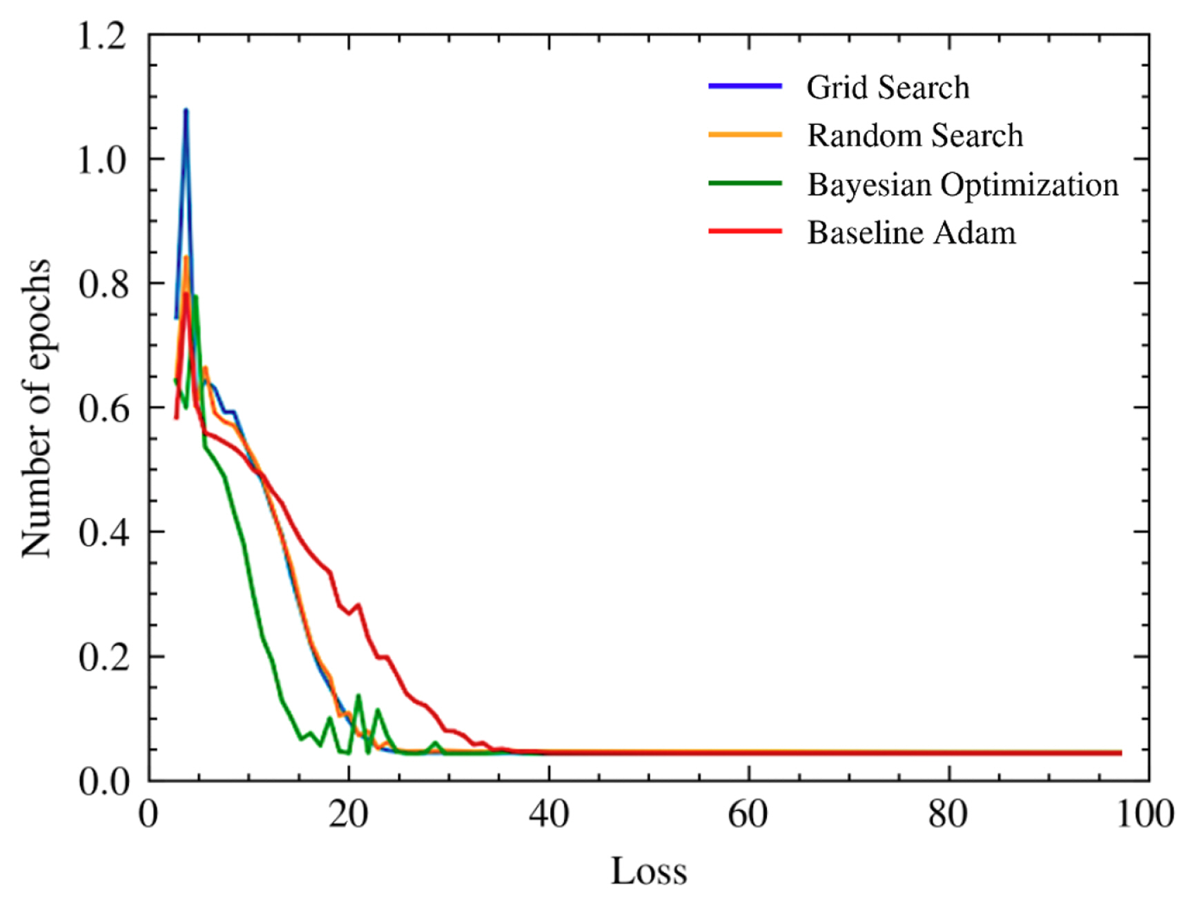
Upon discovering the optimal set of hyper-parameters through the methods mentioned above, we proceeded to extract the latent features correlating with minimal loss during the second experiment’s phase. Additionally, this section revisits the recommended default settings cited earlier. As illustrated in Figure 5, although the minimum loss differential between Bayesian optimization and Grid search was marginal, the convergence of classification loss was markedly swift for the Bayesian method. This rapid convergence did not significantly alter the classification loss when compared to the other methods.

Table 6 furnishes insights into the classification accuracies achieved using the same MLP classifier for anomaly detection. Repeated over 10 trials to ensure robust average performance metrics, these experiments suggest that Bayesian optimization not only accelerates convergence regarding classification loss but it also achieves a superior average accuracy by a margin of 2 percentage points, despite a slightly higher loss function than Grid search. In contrast, Random search, while achieving low classification loss values, fell short in terms of classification accuracy. This underscores the advantage of Bayesian optimization, that is, a balanced approach where both the speed of loss convergence and the precision of classification accuracy are optimized, leading to superior predictive performance when compared to other hyper-parameter tuning methods.

4 Conclusion and Future Work

This study primarily concentrates on improving the process of feature extraction from time-series data by using 1D-CAE. The objective is to enhance the accuracy of anomaly identification in the context of machine health diagnostics. The essential element of this enhancement lies in introducing Bayesian optimization for hyper-parameter tuning, which has been carefully devised to minimize the loss function of the 1D-CAE model. This methodology incorporates a novel modified form of the adjusted hybrid stopping criterion that builds upon the conventional hybrid stopping criteria. It functions as a dynamic measure to determine superior values of the loss function or accelerate the experimental process when favorable outcomes of the loss function are detected. The adjustment entails altering the EI value to fine-tune the balance between the mean and variance in the posterior distribution, hence enhancing the conclusiveness of the experiment.

Bayesian optimization has emerged as a leading approach when compared to conventional hyper-parameter search methods, such as Grid search and Random search that have been commonly used in traditional machine learning frameworks. The results exhibit an accelerated reduction in the loss function as compared to the Random search method. Surprisingly, despite Grid search achieving a somewhat lower loss function, Bayesian optimization demonstrated fast convergence to near-optimal loss function values, with a speed that was 53 times faster.

Empirical evidence supports the assumption that a decrease in the loss function of the model is associated with a more compact representation of the key features of the original dataset in the latent space. As a result, the use of a reduced loss function results in an augmented level of classification accuracy during the succeeding phase of supervised learning. Therefore, by using Bayesian optimization in the process of feature extraction under the framework of 1D-CAE, we are able to achieve improved results while considering the limitations of time and computational resources.

Moreover, the endeavor to optimize hyper-parameters for minimizing the loss function, which is referred to as auto machine learning (AutoML), poses significant difficulties in the field of anomaly detection. This is mostly attributed to the limited availability of publically accessible datasets in this domain. This underscores the need for ongoing innovation within these parameters. Continued investigation is essential to enhance the effectiveness of Bayesian optimization and to improve its ability to extract features for quick and accurate identification of anomalies in time-series data, particularly under AutoML framework.

Declarations

Funding

This work was supported by the Technology Innovation Program (20015756, Development of Fuel Cell Highly Durable Operation Technique for Fuel Cell Powered Heavy Duty Vehicle) funded by the Ministry of Trade, Industry & Energy (MOTIE, Korea)

Fig. 1

Proposed Framework for Bayesian optimization based 1D-CAE architecture

Fig. 2

Schematic of the 1D-CAE architecture

Fig. 3

Autoencoder structure

Fig. 4

Bearing test rig

Fig. 5

Training loss comparison between models

Table 1

Comparison between hybrid stopping criteria and adjusted hybrid stopping criteria

	Hybrid stopping criteria	Adjusted hybrid stopping criteria
	H₀:μ(λ) > f(λ⁺)	H₀:μ(λ) = f(λ⁺) H₁:μ(λ) > f(λ⁺)
Best point	target function before Φ(γ (λ)) < α	target function to be p-value of γ (λ) < α
Measures	Φ(γ(λ))=0.5+0.5×erf(γ(λ)2)	p-value=0.5-0.5×erf(\|γ(λ)\|2)

Table 2

Hyper-parameter search space of grid search

Grid search
Step size	β₁	β₂
0.0001	0.8	0.9
0.002575	0.8475	0.92475
0.00505	0.895	0.9495
0.007525	0.9425	0.97425
0.01	0.99	0.999

Table 3

Hyper-parameter search space of random search and bayesian optimization

	Random search	Bayesian optimization
Step size	(0.0001, 0.001)	(0.0001, 0.001)
β₁	(0.8, 0.99)	(0.8, 0.99)
β₂	(0.9, 0.999)	(0.9, 0.999)

Table 4

Sensitivity analysis result of amount of improvement ɛ

ɛ	Hybrid stopping criteria	Adjusted hybrid stopping criteria
0.0	0.0139	0.0122
0.2	0.149	0.0123
0.4	0.0138	0.0122
0.6	0.0136	0.0135
0.8	0.0138	0.0137
1.0	0.0138	0.0121

Table 5

Loss and training time comparison

	Grid	Random	Bayesian
Min loss	0.0111	0.0128	0.0121
Time	159 min 26 sec	11 min 26 sec	3 min 16 sec

Table 6

Accuracy comparison

	Grid	Random	Bayesian	Default Parameter
Accuracy (%)	86	81	89	87
Average Accuracy (%)	88	79	90	87

Algorithm 1

Bayesian optimization with prior and posterior updating

1:	Initialize prior distribution p(w)
2:	for t = 1,2, ... do
3:	Find x_t by optimizing the acquisition function u over function f xt=argmaxx∈Au(x\|D1:t-1)
4:	Sample the objective function: y_t = f(x_t)
5:	Augment the data D₁_:t = D₁_:t_{– 1}, (x_t, y_t)
6:	Calculate likelihood p(D_1:_t\|w) based on data D_1:_t and current w
7:	Update prior distribution to become the posterior distribution using Bayes’ theorem: p(w∣D1:t)=p(D1:t\|w)p(w)p(D1:t)Set p(w)=p(w\|D1:t)
8:	Update the posterior of the surrogate model f.
9:	end for

References

1. Längkvist, M., Karlsson, L. & Loutfi, A. (2014). A review of unsupervised feature learning and deep learning for time-series modeling. Pattern Recognition Letters, 42, 11–24.

2. Huang, H., Hu, X., Zhao, Y., Makkie, M., Dong, Q., Zhao, S., Guo, L. & Liu, T. (2017). Modeling task fMRI data via deep convolutional autoencoder. IEEE Transactions on Medical Imaging, 37(7), 1551–1561.

3. Makkie, M., Huang, H., Zhao, Y., Vasilakos, A. V. & Liu, T. (2019). Fast and scalable distributed deep convolutional autoencoder for fMRI big data analytics. Neurocomputing, 325, 20–30.

4. Tao, S., Zhang, T.Yang, J.Wang, X. & Lu, W. (2015). Bearing fault diagnosis method based on stacked autoencoder and softmax regression. In: Proceeding of the 2015 34th Chinese Control Conference (CCC); pp 6331–6335.

5. Sun, W., Shao, S., Zhao, R., Yan, R., Zhang, X. & Chen, X. (2016). A sparse auto-encoder-based deep neural network approach for induction motor faults classification. Measurement, 89, 171–178.

6. Meng, Z., Zhan, X., Li, J. & Pan, Z. (2018). An enhancement denoising autoencoder for rolling bearing fault diagnosis. Measurement, 130, 448–454.

7. Masci, J., Meier, U.Cireşan, D. & Schmidhuber, J. (2011). Stacked convolutional auto-encoders for hierarchical feature extraction. In: Proceedings of the Artificial Neural Networks and Machine Learning–ICANN 2011: 21st International Conference on Artificial Neural Networks, Part I 21; pp 52–59.

8. Du, B., Xiong, W., Wu, J., Zhang, L., Zhang, L. & Tao, D. (2016). Stacked convolutional denoising auto-encoders for feature representation. IEEE Transactions on Cybernetics, 47(4), 1017–1027.

9. Liu, X., Zhou, Q., Zhao, J., Shen, H. & Xiong, X. (2019). Fault diagnosis of rotating machinery under noisy environment conditions based on a 1-D convolutional autoencoder and 1-D convolutional neural network. Sensors, 19(4), 972.

10. Bergstra, J., & Bengio, Y. (2012). Random search for hyper-parameter optimization. Journal of Machine Learning Research, 13(2), 1–25.

11. Jones, D. R., (2001). A taxonomy of global optimization methods based on response surfaces. Journal of Global Optimization, 21, 345–383.

12. Lorenz, R., Monti, R. P., Violante, I. R., Faisal, A. A., Anagnostopoulos, C., Leech, R. & Montana, G. (2015). Stopping criteria for boosting automatic experimental design using real-time fMRI with Bayesian optimization. arXiv preprint arXiv:1511.07827.

13. Rumelhart, D. E., Hinton, G. E. & Williams, R. J. (1986). Learning representations by back-propagating errors. Nature, 323(6088), 533–536.

14. Hochreiter, S., (1998). The vanishing gradient problem during learning recurrent neural nets and problem solutions. International Journal of Uncertainty, Fuzziness and Knowledge-Based Systems, 6(02), 107–116.

15. He, K., Zhang, X.Ren, S. & Sun, J. (2016). Deep residual learning for image recognition. In: Proceedings of the IEEE Conference on Computer Vision and Pattern Recognition; pp 770–778.

16. Wickramasinghe, C. S., Marino, D. L. & Manic, M. (2021). ResNet autoencoders for unsupervised feature learning from high-dimensional data: Deep models resistant to performance degradation. IEEE Access, 9, 40511–40520.

17. Kingma, D. P., & Ba, J. (2014). Adam: A method for stochastic optimization. arXiv preprint arXiv:1412.6980.

18. Golovin, D., Solnik, B.Moitra, S.Kochanski, G.Karro, J. & Sculley, D. (2017). Google vizier: A service for black-box optimization. In: Proceedings of the 23rd ACM SIGKDD International Conference on Knowledge Discovery and Data Mining; pp 1487–1495.

19. Kim, S., Park, S., Kim, J.-W., Han, J., An, D., Kim, N. H. & Choi, J.-H. (2016). A new prognostics approach for bearing based on entropy decrease and comparison with existing methods. Proceedings of the Annual Conference of the PHM Society, 8(1), https://doi.org/10.36001/phmconf.2016.v8i1.2540.

20. Qiu, H., Lee, J., Lin, J. & Yu, G. (2006). Wavelet filter-based weak signature detection method and its application on rolling element bearing prognostics. Journal of Sound and Vibration, 289(4–5), 1066–1090.

Biography

Sungeu Chae received the M.S. degree in 2020 and is currently pursuing the Ph.D. degree in industrial engineering from Hanyang University, Seoul, Republic of Korea. His research interests include prognostics and health management, algorithm, and machine learning.

Biography

Suk Joo Bae received the Ph.D. degree from the School of Industrial and Systems Engineering, Georgia Institute of Technology, in 2003. From 1996 to 1999. He is currently a Professor with the Department of Industrial Engineering, Hanyang University, Seoul, Republic of Korea. His research interests include reliability evaluation of light displays and batteries via accelerated life and degradation tests, predictive maintenance for complex systems, process monitoring using on-line big data. He is a member of the INFORMS. He was an associate editor of the IEEE Transactions on Reliability.