Kim, Nam, Kim, and Lee: Artificial Intelligence (AI)–Based Surface Quality Prediction Model for Carbon Fiber Reinforced Plastics (CFRP) Milling Process
Abstract
The objective of this study is to develop a surface quality prediction model for CFRP milling based on artificial intelligence and enhance the model performance by proposing a novel feature through signal processing and applying it to machine learning algorithms. In this paper, the data-driven approach is applied based on data that is obtained by various sensors such as a two-axis load cell, an acoustic emission (AE) sensor, and an accelerometer, and surface quality is predicted as one of three grades based on surface roughness value. To establish the models, a novel feature, referred to as the tool rotation frequency (TRF) feature, was introduced as well as the conventional wavelet transform (WT) feature. Then, three machine learning algorithms – artificial neural network (ANN), K-nearest neighbor (KNN), and support vector machine (SVM) – are used to construct the surface quality prediction models. Each model is trained with 450 data sets obtained from 45 experimental cases, and their predictive accuracy is evaluated by the k-fold cross validation method. Next, to confirm each model’s robustness, 200 data sets obtained from additional 20 experimental cases designed with untrained conditions are tested. Finally, the monitoring software is developed for visualizing prediction results of the surface grades.
Keywords: Carbon fiber reinforced plastics (CFRP) · Milling process · Machine learning algorithms · Surface quality prediction · Tool rotation frequency (TRF)
1 Introduction
Carbon fiber reinforced plastic (CFRP) composites that are fabricated by combining carbon fiber in a polymer matrix have become popular for high-tech industries, such as the aerospace, automobile, and energy [ 1– 3]. Generally, a CFRP is considered a metal substitute due to its superior properties, such as high strength-to-weight ratio, stiffness, and resistance to corrosion. However, there are several disadvantages that limit the scope of its application substantially while CFRP composites have a variety of advantages. Its representative drawbacks are brittleness and high repair cost [ 4, 5]. To manufacture CRFP parts, although most CFRP products are made in a net shape, they generally need to go through a post-machining process such as milling or drilling for assembly and quality satisfaction [ 6]. However, the CFRP incur severe defects during post-machining processes owing to its certain characteristics such as anisotropy, non-homogeneity, and highly abrasive fibers. The surface defects such as fiber pull-out and uncut fiber are difficult to predict during machining processes. In addition, unexpected internal delamination can occur by thermal softening of the matrix when cutting temperature rises above the glass transition temperature of CFRP [ 7, 8]. Therefore, CFRP machining is known to be challenging to control process quality compared to metal machining [ 9, 10]. Thus, appropriate techniques are required for surface quality monitoring and prediction during CFRP machining process. The influence of machining parameters on CFRP surface quality have been researched for many years, but it is difficult to transfer these findings to actual monitoring of CFRP machining processes. Since it is not easy to fully understand the cutting mechanisms of sudden defects such as burrs, fiber-matrix debonding, and saw-tooth surface morphology, much research about the CFRP machining quality monitoring have been studied using various sensors, signal processing methods, and artificial intelligence algorithms.
Several process signals such as cutting force, acceleration, acoustic emission (AE), and motor current have been applied to achieve monitoring for the CFRP cutting processes [ 11– 15]. Selection of proper signal processing methods to be used according to a specific type of signals is important for the machining process monitoring [ 16]. The most widely applied methods can be divided into the four categories: time domain, frequency domain (fast Fourier transform, power spectral density), time-frequency domain (wavelet transform), and others (entropy, fractal analysis et al.) [ 15, 17]. Through the above-mentioned signal processing methods, several studies related to the CFRP machining process monitoring and machined surface quality prediction are reported. Yashiro et al. measured the cutting temperature using the infrared camera and thermocouple in the end milling process of multidirectional CFRP (MD-CFRP), and compared the results with the quality of the machined surface [ 18]. Prakash et al. predicted the cutting force according to the spindle speed and feed rate in the routing process of MD-CFRP, and predicted the surface roughness and delamination. An artificial neural network (ANN) algorithm was used as a regression model for the prediction [ 19]. Krishnamoorthy et al. predicted the delamination at the exit hole according to the spindle speed, feed per revolution, and tool diameter using ANN algorithm in the drilling process of CFRP [ 20]. Eneyew monitored the tool wear and machining quality using an AE sensor, a accelerometer, a microphone sensor in the CFRP machining, and confirmed the correlation. It was found that the peak value generated according to the time of AE sensor and accelerometer has correlation with the machined surface [ 21]. Li et al. investigated the effects of fiber cutting angles on machining surface quality as well as the corresponding milling force signal features based on the time-, frequency-domain and wavelet analysis methods during the CFRP milling. The results show that the cutting force increased significantly for high-frequency component energy percentage according to fiber cutting conditions. In addition, it was confirmed that the fluctuation trend of power percentage for frequency band of 1,500–2,500 Hz can be used as a monitoring index for indicating the CFRP machining surface roughness [ 22]. As mentioned in those studies, efforts have been made to analyze the correlation between sensor signals and surface quality and to find features that can be used as an index for CFRP machining monitoring. However, there are no researches of developing models for predicting CFRP milling surface quality using a new monitoring index which has meaningful process information for being applied to AI algorithms. In particular, the quality prediction model in other research was not tested for untrained process cases after the model was built. The robustness of the model in terms of practical aspects was not confirmed [ 23]. The objective of this study is to develop a surface quality prediction model for CFRP milling based on machine learning algorithms, and to demonstrate the enhanced model performance by proposing a new feature - tool rotation frequency (TRF). The data-driven approach by collecting a large amount of data from various sensors such as the two-axis load cell, AE sensor, and accelerometer. The new feature - TRF - was extracted from the collected data as well as conventional wavelet transform (WT) feature for a comparison. For machine learning algorithms, artificial neural network (ANN), K-nearest neighbor (KNN), and support vector machine (SVM) - were used to build the surface quality prediction model of CFRP milling process. Those models predict the CFRP surface quality as one of three grades. A prediction accuracy of the trained 18 models is evaluated through a k-fold cross-validation process. In addition, a robustness of the 18 models was tested by applying untrained new machining conditions with new five types of milling tools. Finally, the best model is used for developing the software interface to effectively monitor and predict the surface quality during CFRP milling process.
2 Experiments and Data Collection
2.1 Experimental Setup
In this paper, a multi-directional CFRP (MD-CFRP) composite was used as the workpiece for the milling process. The size of the workpiece was 34 × 50 × 3 mm 3. The MD-CFRP workpiece was fabricated with 10-ply. The stacking sequence was [90/ 135/ 135/ 0/ 45/ 45/ 0/ 135/ 135/ 90°] s and is schematically shown in Fig. 1. Properties of the carbon fiber and the prepreg is listed in Table 1. The prepreg with a carbon fiber of T700 (Toray Composite Materials America, Inc.) was used and the resin was epoxy (SKYFLEX K51). The three-axis horizontal machine tool system is built for the CFRP milling experiments, and it consisted of three DC-motor driven linear stages (MX80S, Parker-Hannifin Corporation), an electric spindle (E-800Z, Nakanishi) and a programmable multi-axis controller (CEM 104, Delta Tau Data Systems). Fig. 2 shows the experimental setup for CFRP milling process. Four sensors such as the two-axis (X-axis and Y-axis) load cell (MAS110-5LLT, LOADTEC), AE sensor (PICO, MISTRAS), and accelerometer (Type 4394, B&K) were used. The DAQ chassis (NI cDAQ-9178) and DAQ module (NI 9232) were set to obtain sensor data, and the sampling rate was 50,000 Hz. The MD-CFRP composite workpiece was mounted on the two-axis load cell. The AE sensor and accelerometer were attached on the workpiece. The milling tool was mounted on the electric spindle.
For lubrication, the customized nano-solid dry lubrication module that is composed of an air cleaning duct (ZERO SMOG 4V, Weller), an air compressor (PAB 42T3-50F, Power Air), a drain filter (WD-02, Win & Tech Korea), and a precision regulator (IR1010-01BG, SMC) is installed [ 25]. Graphene nanoplatelets classified as xGnP H-5 manufactured by XG SCIENCE were used as nano-solid lubricants. The xGnP H-5 had an average particle size (APS) of 5 μm, a thickness of 15 nm, and specific surface area (SSA) of 50–80 m 2/g. This nanoparticle had a form of stacks of thin two-dimensional (2D) sheets, and which could have a sliding effect by reducing friction at the tool-workpiece interface through lubrication effect [ 26, 27]. An external spray nozzle with an internal diameter of 3 mm was used for spraying the nanoparticles to cutting zone, which was located at 20 mm away from the workpiece with a spraying feed angle of 10° with respect to the workpiece. This lubrication method was applied in all experimental cases in this study. Table 2 summarizes the experimental conditions.
2.2 Experimental design
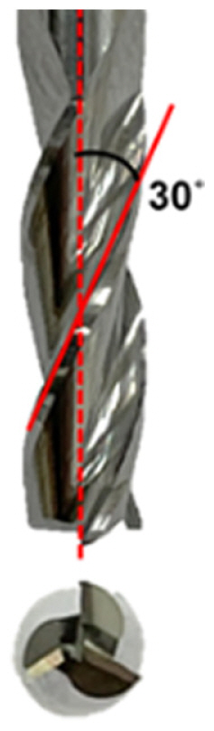
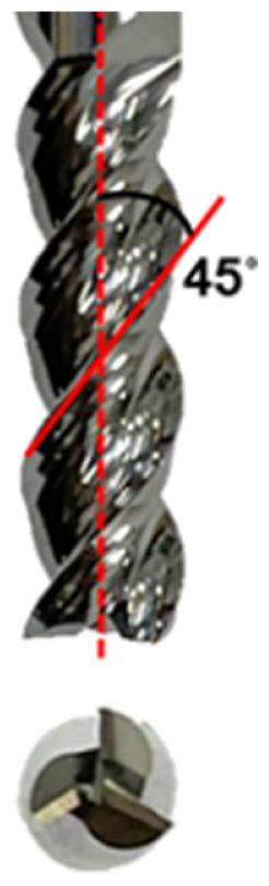
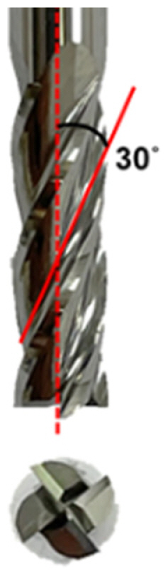
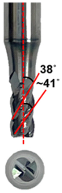
The CFRP milling experiments were designed for a surface quality model construction and a robustness test. For the model construction, 45 experimental cases were designed considering five types of tool geometry, three levels of spindle speed, and three levels of feed rate, and ten data sets were obtained in each experimental case. Therefore, 450 data sets were acquired. The specifications of five types of the tools are summarized in Table 3. Among the tools given Table 3, T2, T4, T6, T8, and T9 were the model construction. Table 4 summarizes the designed experimental cases for the model construction. The number of passes during milling process was five in each case. The surface roughness of the milling surfaces were measured after five milling passes. After the experiments for the model construction, additional experiments were designed for the robustness test. In the robustness test, the surface quality prediction model was applied to the milling process with tools that were not used for the model construction. Thus, total 10 types (T1~T10) of milling tools were used by adding new five tools. They are also shown in Table 3. Herein, 20 experimental cases for the robustness test were designed, and 10 data sets were obtained in each case. Therefore, 200 data sets were used for robustness test, and the experimental design is presented in Table 5.
3 Surface Quality Analysis
Surface quality was examined by obtaining 3D profile data using a 3D laser microscope (VK-X series, Keyence). To quantitatively analyze the surface quality, the arithmetical mean height (Ra) surface roughness was measured from the obtained 3D profile data.
The surface roughness was evaluated by measuring transverse roughness and longitudinal roughness. The transverse roughness refers to roughness measured perpendicular to the cutting feed direction. The longitudinal roughness refers to roughness measured parallel to the cutting feed direction. The transverse and longitudinal roughness have been investigated together for more precise analysis of CFRP surface [ 28, 29]. When measuring the surface roughness, 10 parts of the milled surface were segmented and both transverse and longitudinal surface roughness values were obtained. Fig. 3 shows the sample image of milled CFRP surface in which 10 segmented parts are denoted yellow color. Each part was 1.5 mm apart from each other. In transverse roughness, a cut-off length of 0.8 mm and a measurement length of 2.8 mm for 11 lines were obtained, and the measured values in each 11 lines were averaged. In longitudinal roughness, a cut-off length of 0.8 mm and a measurement length of 1.2 mm for 15 lines were obtained, and the measured values in each 15 lines were averaged. For the surface quality analysis, larger one between the transverse and longitudinal roughness of each data set was selected as the final surface roughness value.
Surface quality was classified into three grades based on surface roughness values. A value of CFRP surface roughness less than 3.2 μm is set as Grade 1. This is the standard required value in aerospace industry [ 30]. CFRP surface roughness between 3.2 and 6.0 μm is set as Grade 2 with reference to the international tool manufacturer’s process stability standards [ 31]. CFRP surface roughness higher than 6.0 μm was classified as Grade 3, wherein the surface quality is not good even when observed visually. The samples of 3D profiles of the milled surface classified as Grades 1, 2, and 3 are shown in Fig. 4.
Fig. 5 shows the classification results of 450 data sets into three grades according to their surface roughness values. Grades 1, 2, and 3 are expressed as green, yellow, and red, respectively. Among the 450 sets, 140 (31.1%) were of Grade 1, 95 (21.1%) were of Grade 2, and 215 (47.8%) were of Grade 3. This distribution was judged to be appropriate for developing the surface quality prediction model. These grade values were assigned to the output layer while training the model.
4 Feature Extraction and Selection
The x-axis force, y-axis force, acoustic emission, and acceleration signals were used to extract and select features that were input to the surface quality prediction models. In this study, two types of features were extracted. The first type was extracted using a conventional wavelet transform (WT) method. The second type was a novel feature defined as the tool rotation frequency (TRF) feature, which was proposed to improve the robustness of the surface quality prediction models.
4.1 Wavelet Transform (WT) Feature
The wavelet transform (WT) is a widely used feature extraction tool for processing signals. It provides a high frequency resolution at low frequencies, and a high time resolution at high frequencies in contrast to short-time Fourier transform (STFT). It is specialized for non-stationary signals whose frequency information changes with time [ 32]. The mother wavelet is selected as Daubechies wavelet (db4) and an 8-level wavelet decomposition was conducted. Fig. 6 shows the 8-level wavelet decomposition diagram. The analysis frequency band is 0–25,000 Hz because the sampling rate of sensor data was set to 50 kHz. The a1–a8 are low pass approximation coefficients and d1–d8 are high pass detail coefficients. The raw signal can be expressed by: In this study, 9 coefficient signals (s, d1, d2, d3, d4, d5, d6, d7, and d8) were obtained through 4 sensors and 10 statistical values were extracted from each coefficients signal. Thus, 360 features were extracted.
The calculation equations for each statistical features are given in Table 6. They represent the energy, the distribution, and the waveform of signal. The features of Max, Min, Mean, and Root mean square (RMS) represent the magnitude of energy of the signal. The features of Variance, Skewness, and Kurtosis explain the distribution of the signal. The features of Shape factor, Crest factor, and Impulse factor are correlated with the waveform of the signal. A feature selection process is needed to improve the classification performance and to reduce the training time of AI algorithms. A statistical approach is used to select critical features. Z-test, T-test, and analysis of variance (ANOVA) are popular methods. Z-test is unsuitable to use on the sampled data because it is only applicable when the population is known. Therefore, an ANOVA was used. This method distinguishes between groups, similar to a T-test. However, it differs from a T-test in that the ANOVA can find the difference between the means among three or more groups, not just two groups [ 33]. Through the ANOVA approach, the P-values for each WT feature were calculated. The P-value is the significance level for t-statistics. The null hypothesis, i.e., that the mean values of the three groups are equal, is commonly rejected when the significance level is less than 0.05 (5%) and 0.01 (1%). These levels mean good evidence for statistically significant difference against the null hypothesis. In addition, when a significance level is less than 0.001 (0.1%), the P-value means very strong evidence against the null hypothesis. In this study, a significance level of 0.001 (0.1%) was determined as the criteria in the feature selection process. As a result, 213 WT features with the P-value less than 0.001 were selected as the final features to be used in machine learning out of the 360 extracted features. Table 7 summarizes the representative 30 top-ranked features with the lowest significance levels among the 213 selected features.
4.2 Tool Rotation Frequency (TRF) Feature
In the machining process, a tool rotation frequency and its harmonics are known to contain valid information. Many researchers have studied the machining process characterization using a tool rotation frequency [ 22, 34, 35]. However, there was no case in which these characteristics were numerically defined through signal processing and used as input variables for machine learning algorithms. Thus, the TRF feature was introduced to maximize the robustness of the surface quality prediction model, maintaining high performance even under untrained new machining conditions. The TRF feature was intended to subdivide the characteristic frequency information attributed to the physical phenomenon of tool rotation during mechanical machining processes. These properties, consisting of bands of harmonics of the tool rotation frequency, contain meaningful information related to the cutting mechanism.
For tool rotation frequencies, the magnitude of the dominant peak depends on the feed rate and the type of tool. The number of harmonics of the tool rotation frequency obtained in a given frequency band also depends on the spindle rotation speed.
In this study, the TRF features were extracted from one sensor as 110 representative values and applied to the machine learning models regardless of machining conditions, tool rotation frequency, and its harmonic information. Fig. 7 illustrates five steps of obtaining such a feature for the sample case - Run 7 in Table 4. A descriptions of each step are given below:
In one data set (sampling length: 1.5 mm), 56,250 indices were obtained as raw data from the AE sensor at a sampling rate of 50,000 Hz and a feed rate of 80 mm/min. To confirm valid information through the tool rotation frequency during the machining process, it was converted from the time domain to the frequency domain. Power spectral density (PSD) analysis was conducted. As this approach is independent of frequency resolution, it is useful to compare vibration levels of the signals having different numbers of data indices. That is, PSD is not dependent on a sample time as compared to the time-dependent FFT method [36]. In the PSD domain, all bands with TRF harmonics as the median were constituted, and 78 bands were defined by diving the frequency band (25,000 Hz) with the tool rotation frequency (316.7 Hz). The indices in each band were converted into one statistical value and a single TRF curve consisting of these values was obtained. Then, 10 TRF curves were obtained because 10 types of statistical values given in Table 6 were used. These TRF curves complement the characteristics that the number of TRF bands is not the same in the case of different spindle rotation speeds.
In this study, 4 sensors were used for feature extraction, and 10 TRF curves and one time domain profile were obtained from one sensor. Finally, 440 features were extracted. In addition, the TRF feature complement the characteristics of the WT method, which has low frequency resolution at the high frequency band. This is because large peaks could be frequently found in the high frequency band rather than the low frequency band as many carbon fibers are cut very quickly by the brittle fracture mechanism during the CFRP milling process.
To select the critical TRF features that better distinguish three surface grades, the ANOVA method, as in the selection of the WT features, was used. The P-values for each TRF feature were obtained. A significance level of 0.001 (0.1%) was set as the criteria in this feature selection process. 403 TRF features with the P-value less than 0.001 were selected out of the 440 extracted features. The representative 30 top-ranked features are summarized in Table 8.
5 Development of Surface Quality Prediction Model
To develop the surface quality prediction model, three representative machine learning algorithms for classification such as artificial neural network (ANN), K-nearest neighbor (KNN), and support vector machine (SVM) were used. The model validation was conducted using a k-fold cross validation method, and its robustness was tested under new machining conditions.
For training each machine learning based model, two types of features were prepared as the input variables: WT feature and TRF feature. For the two types of features, all features with P-value less than 0.001 were used, and among them, top-ranked 10 and top-ranked 30 features were also used for comparatively evaluating the model performance. Thus, six cases of input variables composed of WT features and TRF features were used: 10 WT features, 30 WT features, 213 WT features, 10 TRF features, 30 TRF features, and 403 TRF features. As the output responses, the numerical values of 0, 1, and 2 were assigned to surface Grades of 1, 2, and 3, respectively.
5.1 Machine Learning Algorithms
Artificial neural network (ANN) is a computational model created by applying the concepts of a biological neural network. The ANN has many artificial neurons called processing units, which are interconnected by nodes. These processing units are composed of input and output nodes. The input nodes receive various forms and structures of information based on an internal weighting system, and the neural network attempts to learn about the information presented to produce one output result. The ANN uses a set of learning rules called back propagation, an abbreviation for backward propagation of error, to perfect its output results. Its major objective is to modify values of weight and bias, using feedback on evaluation of errors [ 37]. In this study, four layers were designed for the ANN algorithm. Fig. 8 shows its schematic diagram. The first layer is the input layer containing the selected features assigned to the ANN model. The second and third layers are hidden layers that each have 16 nodes. The fourth layer is the output layer. The surface grades were supplied to the output layer during supervised training of the algorithm. The activation function of the ANN was a rectified linear unit (ReLU), and the hyper-parameters are as follows: learning rate—0.0001; iteration—2,000.
K-nearest neighbor (KNN) is a methodology that predicts new data with information from the k nearest neighbors among existing data. This is in contrast to the model-based learning because it performs classification or regression using only observation without model creation. The KNN is not substantially affected by noise embedded in the training data. It is quite effective if the number of training data is large. However, it takes a long time to calculate because all distances between new observations and each training data have to be measured. The hyper parameters of KNN are the number of neighbors to search (K) and the distance measurement method. When (K) is small, it overfits the regional characteristics of the data (overfitting). Conversely, if it is very large, the model tends to be over-normalized (i.e., underfitting) [ 38]. In this study, the number of neighbors to search through (K) was set as ‘5’ and the measuring method was ‘Manhattan distance’. Support vector machine (SVM) is a classifier designed to maximize the margin between two classes and minimize the error rate. The margin is the distance between two categories obtained with respect to the support vector. In this study, classification into three categories is needed, so the kernel trick was used for non-linear classification. A polynomial kernel with a degree of 3 was applied for establishing the SVM model. The kernel scale γ was ‘auto’.
5.2 Model Development and Validation
The performance evaluation of the models was carried out using the 450 collected data sets i.e., 140 data for Grade 1, 95 data for Grade 2, and 215 data for Grade 3. First, the three AI models were evaluated considering the six cases of input variables composed of WT features and TRF features. A k-fold cross-validation method in which the limited number of data can be used more efficiently was applied to compare the accuracy of each model. In this validation method, 450 original data are randomly distributed to k sub-data groups of an equal size. After that, (k-1) sub-data groups are used for training the model, the remaining single sub-data group d is used for validating the model. This process is repeated for k-times by cyclically changing the validation data set.
In this study, five-fold cross validation was conducted. The accuracy of each fold was obtained by counting the cases in which surface quality grades were correctly diagnosed among 90 validation data sets for each fold. The validation results are presented in Table 9 and total 18 models were compared in terms of an average accuracy. Fig. 9 shows the graph of this results. Overall, the models based on TRF features showed higher validation accuracy for all models regardless of the number of features. It was also demonstrated that the models trained by WT features are greatly affected by the predictive accuracy according to the number of features. The highest accuracy was found in the models trained by 403 TRF feature for KNN algorithm, and the value was 90.22%.
5.3 Robustness Test
After the model validation, additional experiments of 20 cases were conducted for further testing the model. For these test, the entire 450 data sets, used for the model validation process, were applied for training the model. As previously mentioned in Section 2.2, five new tools that were not used in the training process were added for the robustness test. Thus, 10 types of tools were used totally. All machining conditions (spindle speed and feed rate) were designed with new conditions other than those used in the training process. Herein, new 200 data sets were tested for robustness evaluation of the model.
In a same manner for the model validation, the three machine learning-based models were constructed by considering the six cases of input variables composed of WT and TRF features. The results of robustness test are summarized in Table 10 and the 18 models were compared in terms of test accuracy. Fig. 10 shows the graph of these results. The model trained with 10 TRF features and ANN algorithm had the highest prediction accuracy of 81%. By contrast, among WT features, the best model used 30 features, and the prediction accuracy was 77.5%. The models trained by TRF features showed higher prediction accuracy than the models trained by WT features even when being verified with data collected under new test conditions.
In the results of best model performance of ANN with 30 WT features and 10 TRF features, the test accuracy of the 100 data sets with tools used for training model and the other 100 data sets with newly added tool were analyzed in detail. Among the test accuracy of 77.5% for 200 data sets of the model trained with 30 WT features, the test accuracy for 100 data sets with the tool used for training was 81%, and for 100 data sets with the new tool, the test accuracy was 74 %. On the other hand, among the test accuracy of 81 % for 200 data sets of the model trained with 30 TRF features, the test accuracy for 100 data sets with the tool used for training was 81%, and for 100 data sets with the new tool, the test accuracy was 81%. The TRF features maintained a robust prediction performance even when new machining conditions were tested using new tool, but the WT features showed a significantly degraded performance. Therefore, it was confirmed that TRF features could show a relatively more robust performance in the case of untrained new machining environments.
Overall, higher accuracy could be obtained in the ANN- and KNN-based surface quality prediction models than the SVM-based one in the model validation and robustness test. In general, SVM is more advantageous for classifying two classes than three. In the robustness test, the highest accuracy of KNN was lower than that of ANN. Since KNN does not directly create specific models, it can be limited in understanding the relationships between features and classes.
In terms of the number of features, in case of a large number of features, overfitting problems could occur. The ANN could solve this problem by deepening the model structure. The KNN overfits regional characteristics when the hyperparameter k is small. As a result, it is important to find an optimal structure of the model and an appropriate number of features. For application of practical machining environment, the ANN-based surface quality prediction model with high robustness test accuracy was advantageous.
For the 30 WT feature-based model and the 10 TRF feature-based model, the best test performance based on the ANN algorithm was confirmed. The confusion matrices are shown in Fig. 11 to visualize the prediction results. Quality control problems arise when the predicted quality is better than the actual quality, and this cases are highlighted with red box in the confusion matrices. Therefore, TRF feature-based model shows a bit better prediction performance than WT feature-based model. The software interface to monitor and predict the surface quality grades during CFRP milling process was developed using the Python programming language. The graphical user interface (GUI) is shown in Fig. 12. The GUI was designed for visualizing the monitoring information and the results of surface quality grade prediction. It has functions of displaying the raw data and TRF curve that was processed from the raw data. When using the software to predict the CFRP surface quality grades, it is necessary to input the sampling frequency, spindle speed, and feed rate. Based on the input information, the TRF value is calculated from the raw data of the sensors, and this value is used input to the pre-trained ANN model, and the final prediction result is shown as one of Grades 1, 2, and 3. The Grades 1, 2, and 3 are expressed as green, yellow, and red, respectively. In addition, the surface quality prediction for each of 10 sections is enabled while milling one pass of the CFRP surface.
6 Conclusion
In this paper, the machine learning-based surface quality prediction model for CFRP milling process was established by extracting the new feature – TRF. The surface quality grades – Grades 1, 2, and 3 – were defined based on the measured surface roughness (Ra) values.
When developing the models, three machine learning algorithms – ANN, KNN, and SVM – were considered. The novel TRF features were input to the above-mentioned three algorithms, and at the same time, the conventional WT features were input to the algorithms for a comparison.
To evaluate the prediction performances of each model, the validation accuracy was compared after apply the k(5)-fold cross validation method. The highest accuracy was found in the models trained by 213 WT features and 403 TRF features with KNN algorithm, and the validation accuracy value was 90.22%. In addition, the robustness test was applied by introducing the new tools and new machining conditions that were not considered in the training stage. When using the TRF features in the ANN-based model, the test accuracy was 81.0%, which was better than the ANN-based model with the conventional WT features. Finally, the software interface was developed to display raw data of the sensor signals, the processed TRF features, and the surface quality grade prediction results, respectively.
Fig. 1
Stacking sequence of MD-CFRP for milling process 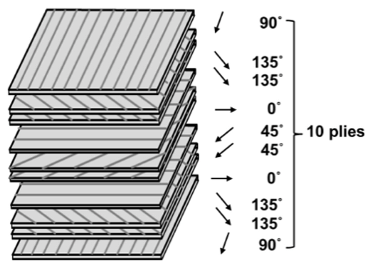
Fig. 2
Experimental setup for CFRP milling experiments 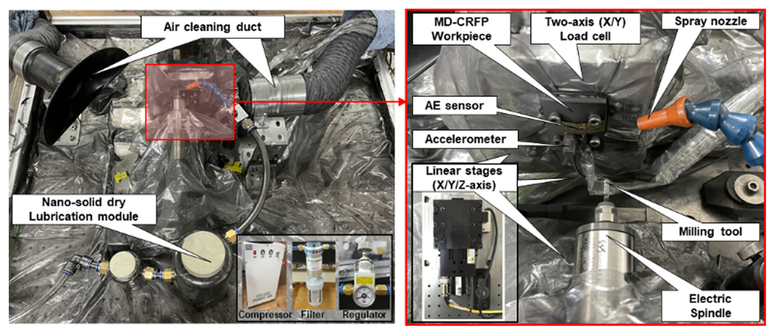
Fig. 3
10 segmented parts of CFRP surface for surface roughness measurement 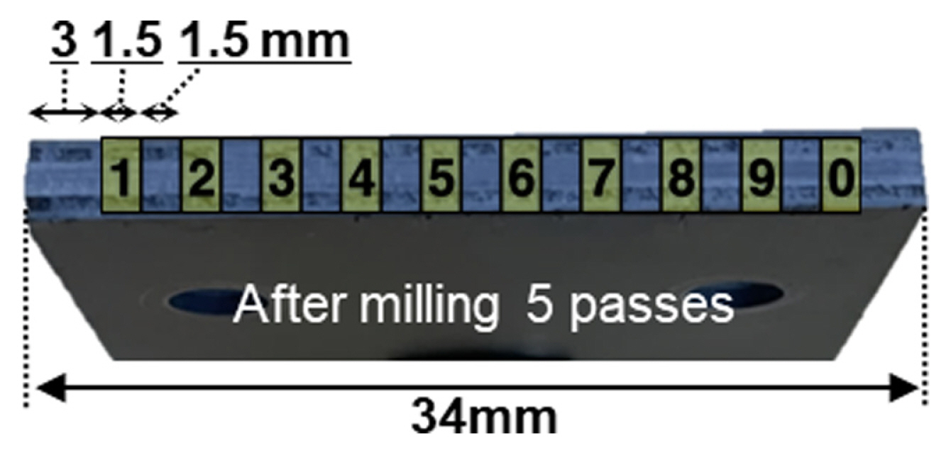
Fig. 4
Samples of 3D profiles of the milled surface classified as Grades 1, 2, and 3 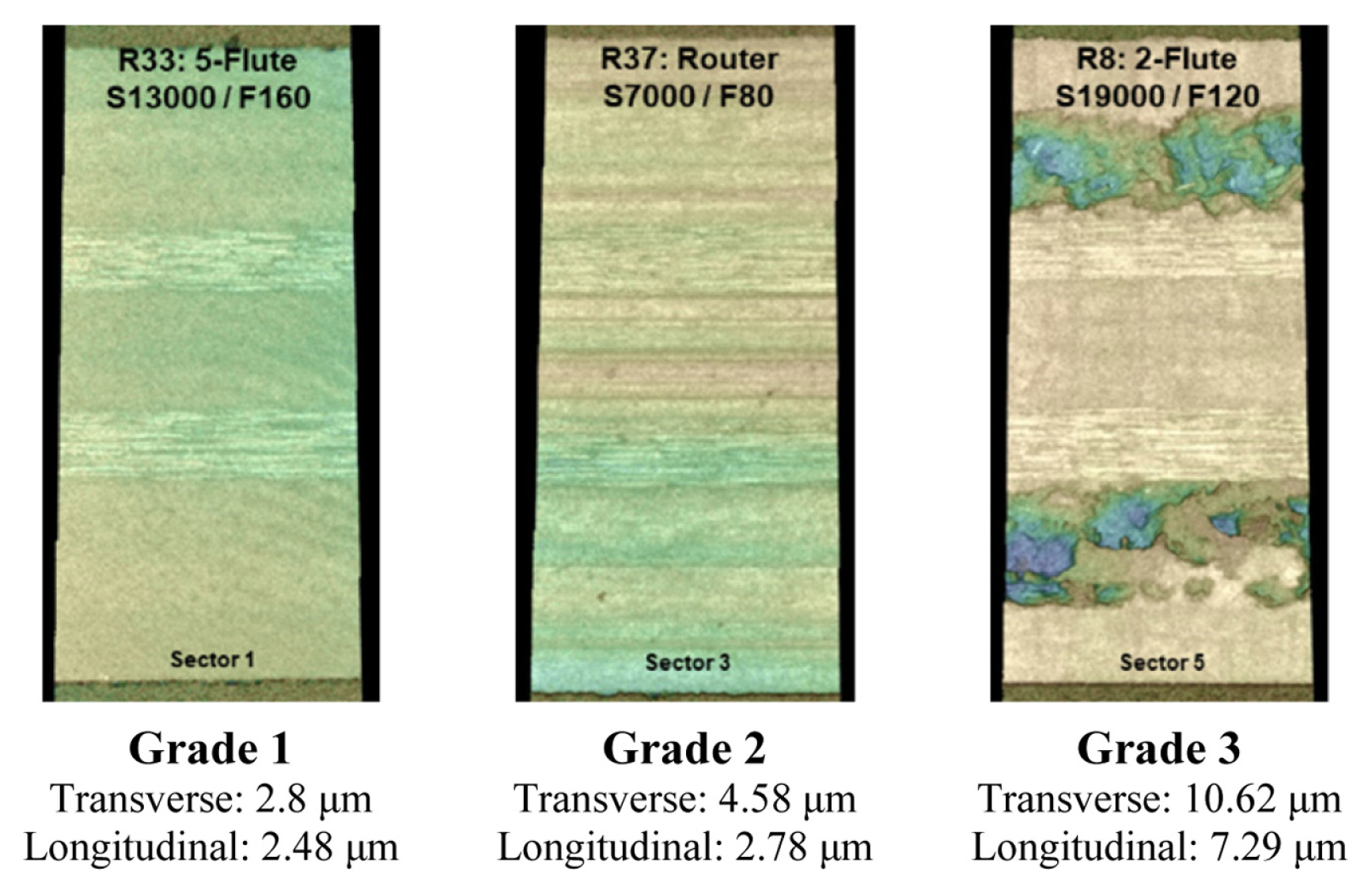
Fig. 5
Surface grade decision in 450 data sets 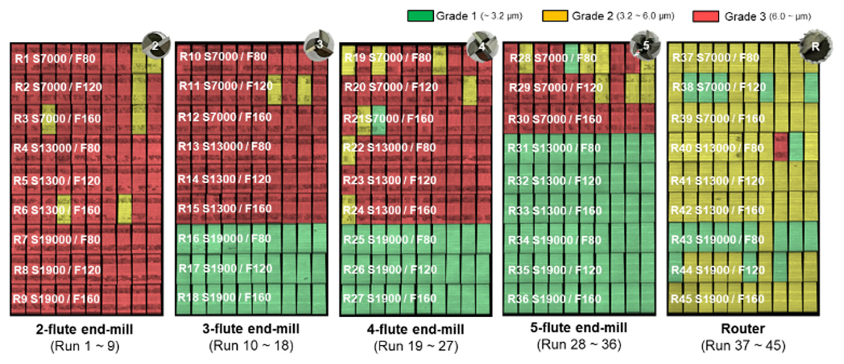
Fig. 6
8-level wavelet decomposition diagram 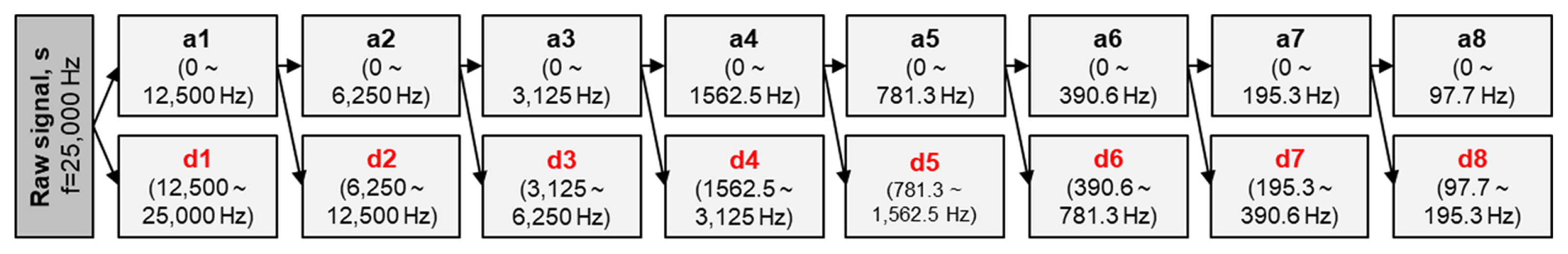
Fig. 7
Schematic illustrations of five steps for obtaining TRF features 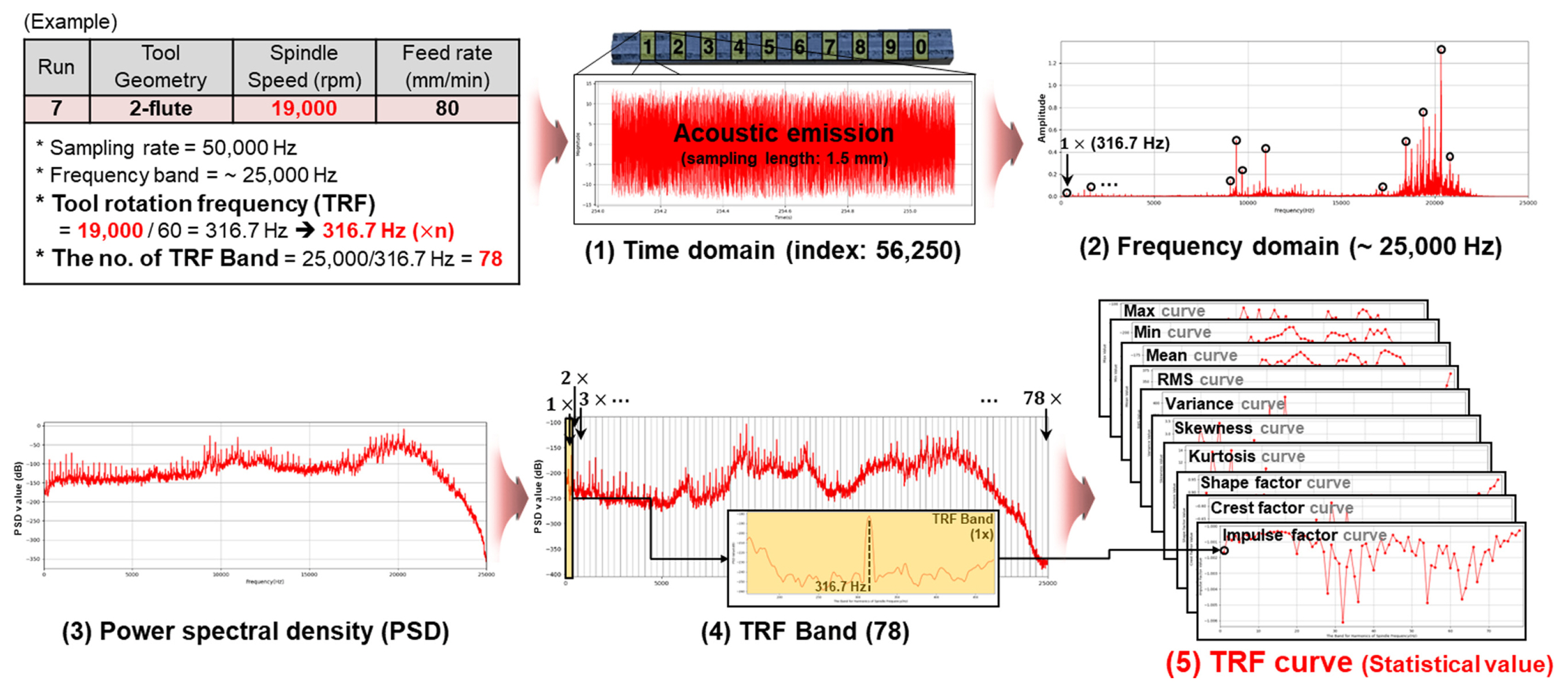
Fig. 8
Schematic diagram of artificial neural network 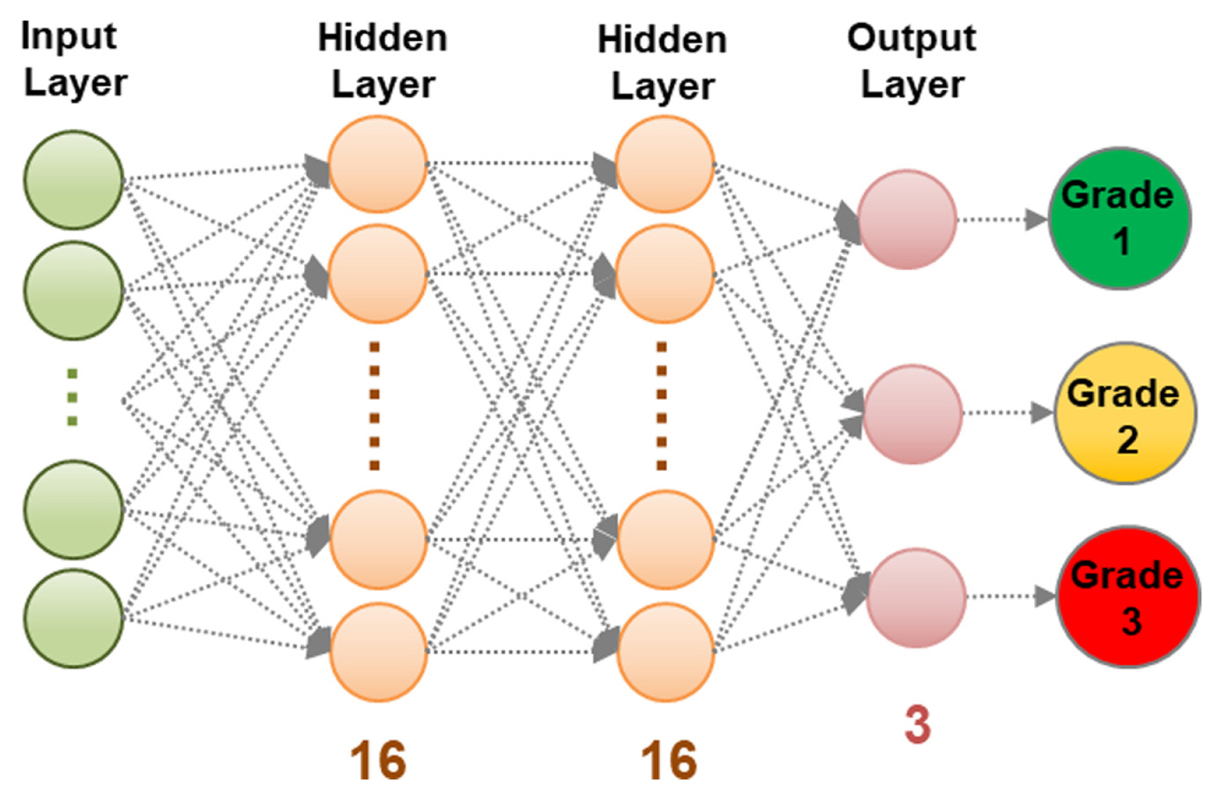
Fig. 9
Average validation accuracy of each model for surface quality prediction 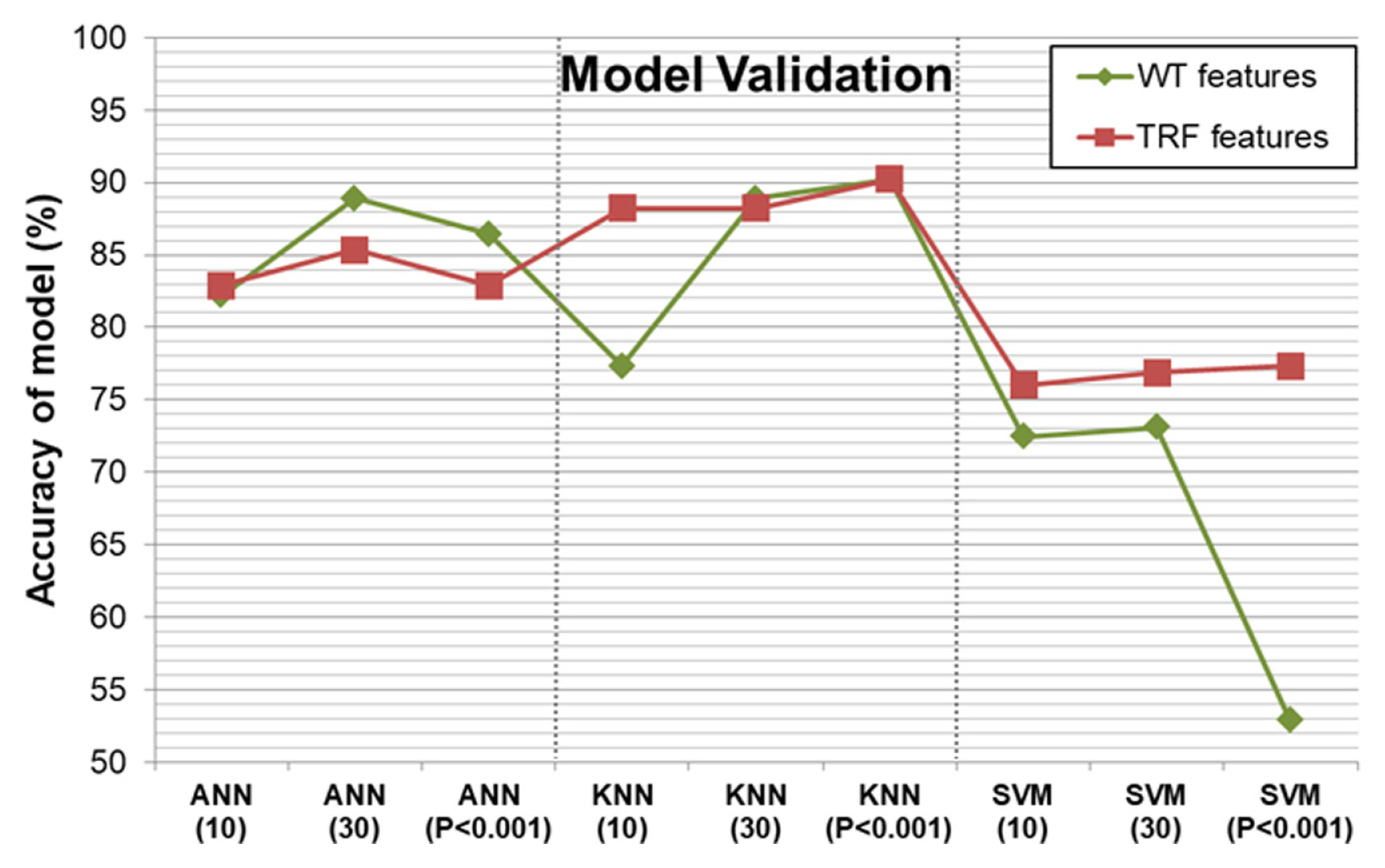
Fig. 10
Accuracy of each model for surface quality prediction during robustness evaluation 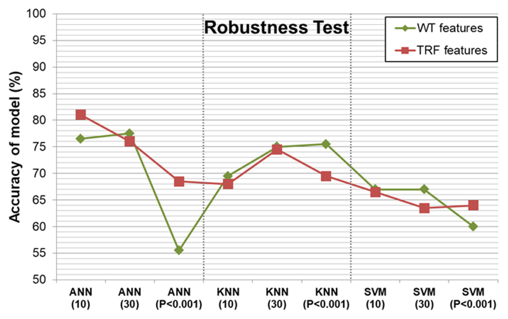
Fig. 11
Confusion matrix of robustness test results 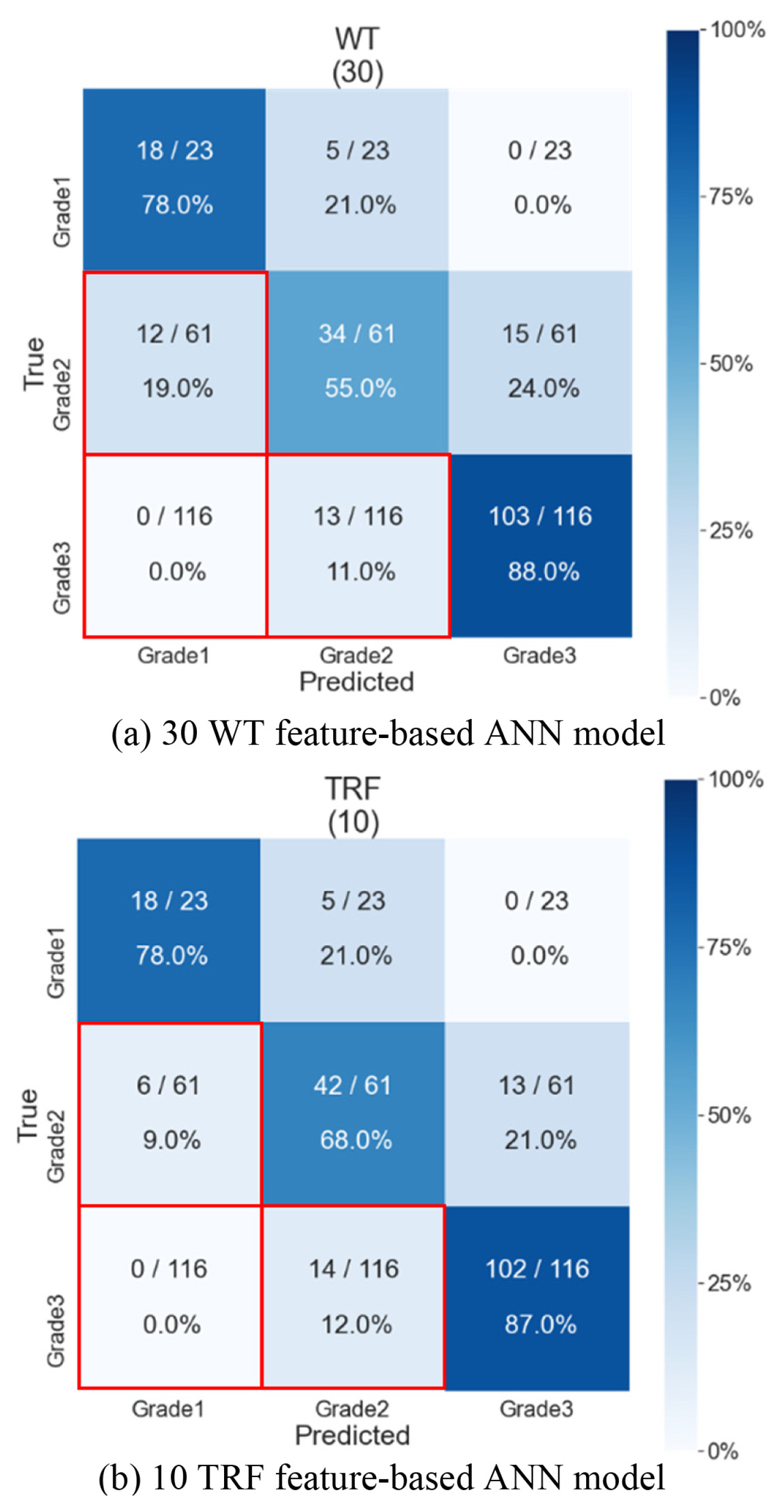
Fig. 12
Snapshot of CFRP milling quality prediction results in the GUI 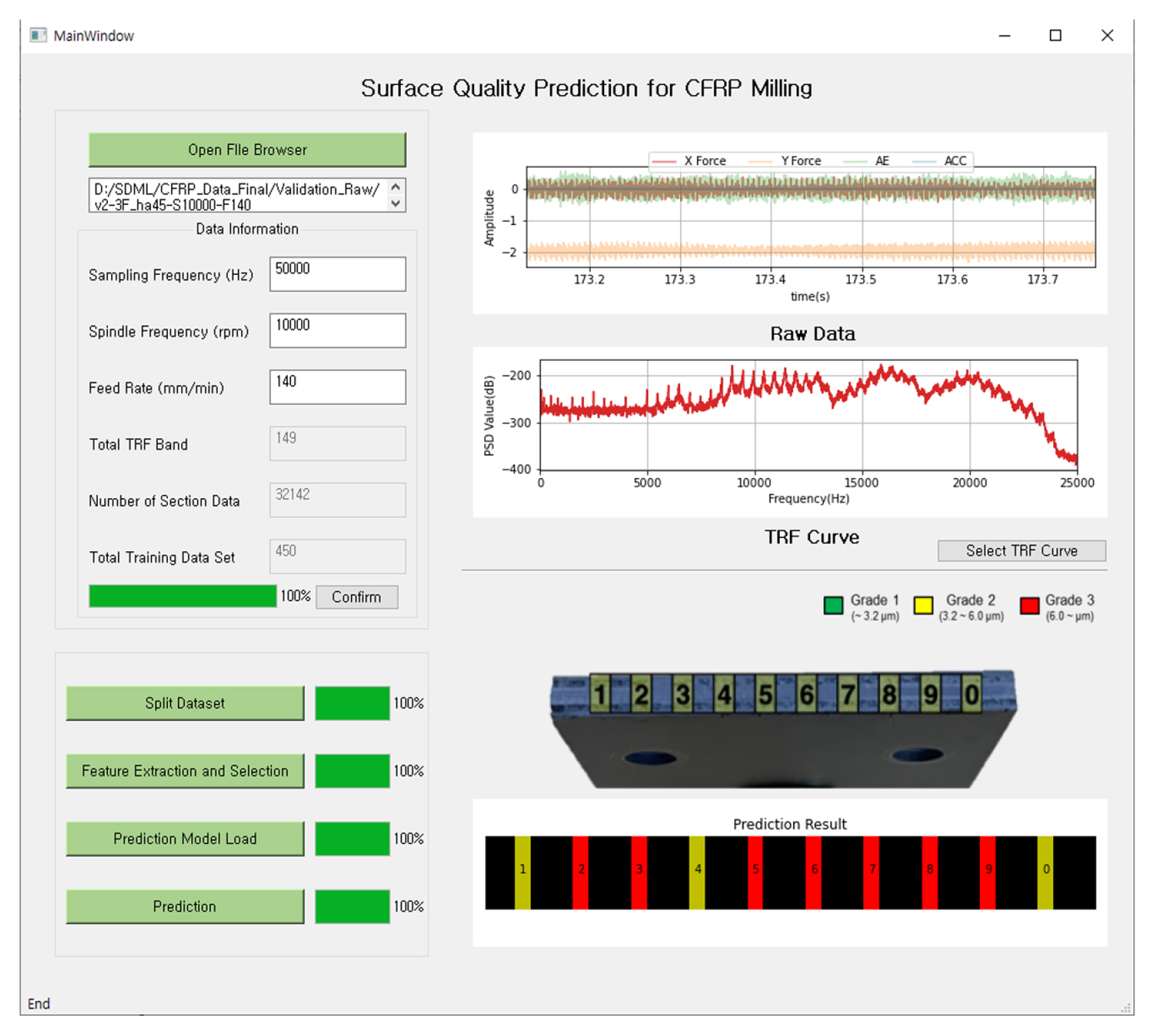
Table 1
Properties of carbon fiber and prepreg [ 24] Adapted from Ref. 24 on the basis of web page
|
Properties |
Information |
|
Standard of carbon fiber |
T700 |
|
Thickness of each ply (μm) |
310 |
|
Tensile strength (MPa) |
4,900 |
|
Tensile modulus (GPa) |
230 |
|
Strain (%) |
2.1 |
|
Density (g/cm3) |
1.80 |
|
Filament diameter (μm) |
7 |
|
Fiber area weight (FAW) (g/m2) |
150 |
|
Fiber volume (%) |
64 |
|
Resin |
Epoxy |
Table 2
Experimental conditions for CFRP milling process
|
Tool |
Carbide end mill (10 types) |
Model construction: T2, T4, T6, T8, T9
Robustness test: T1–T10 |
|
Workpiece |
Material |
MD CFRP |
|
Size (mm3) |
34 × 50 × 3 |
|
Milling |
Type |
Side milling |
|
Number of passes |
5 |
|
Machining conditions |
Spindle speed (rpm) |
Model construction: 7,000/13,000/19,000
Robustness test: 10,000/16,000 |
|
Feed rate (mm/min) |
Model construction: 80/120/160
Robustness test: 100/140 |
|
Radial depth of cut (μm) |
300 |
|
Axial depth of cut (mm) |
3 |
|
Lubrication conditions |
Method |
Nano-solid dry lubrication |
|
Nanoparticles |
xGnP H-5 |
|
Nozzle diameter (mm) |
Φ = 3 |
|
Nozzle angle (°) |
10 |
|
Spray distance (mm) |
20 |
|
Air pressure (bar) |
0.4 |
Table 4
Experimental design for model construction
|
Run |
Tool geometry |
Spindle speed (rpm) |
Feed rate (mm/min) |
|
1 |
2-flute end-mill (T2, Helix angle: 30°) |
7,000 |
80 |
|
2 |
120 |
|
3 |
160 |
|
4 |
13,000 |
80 |
|
5 |
120 |
|
6 |
160 |
|
7 |
19,000 |
80 |
|
8 |
120 |
|
9 |
160 |
|
10 |
3-flute end-mill (T4, Helix angle: 30°) |
7,000 |
80 |
|
11 |
120 |
|
12 |
160 |
|
13 |
13,000 |
80 |
|
14 |
120 |
|
15 |
160 |
|
16 |
19,000 |
80 |
|
17 |
120 |
|
18 |
160 |
|
19 |
4-flute end-mill (T6, Helix angle: 30°) |
7,000 |
80 |
|
20 |
120 |
|
21 |
160 |
|
22 |
13,000 |
80 |
|
23 |
120 |
|
24 |
160 |
|
25 |
19,000 |
80 |
|
26 |
120 |
|
27 |
160 |
|
28 |
5-flute end-mill (T8, Helix angle: 40°) |
7,000 |
80 |
|
29 |
120 |
|
30 |
160 |
|
31 |
13,000 |
80 |
|
32 |
120 |
|
33 |
160 |
|
34 |
19,000 |
80 |
|
35 |
120 |
|
36 |
160 |
|
37 |
Router (T9, Diamond cut) |
7,000 |
80 |
|
38 |
120 |
|
39 |
160 |
|
40 |
13,000 |
80 |
|
41 |
120 |
|
42 |
160 |
|
43 |
19,000 |
80 |
|
44 |
120 |
|
45 |
160 |
Table 5
Experimental design for robustness test
|
Run |
Tool geometry |
Spindle speed (rpm) |
Feed rate (mm/min) |
|
1 |
1-flute end-mill (T1, Helix angle: 25˚) |
10,000 |
140 |
|
2 |
16,000 |
100 |
|
3 |
2-flute end-mill (T2, Helix angle: 30˚) |
10,000 |
140 |
|
4 |
16,000 |
100 |
|
5 |
2-flute end-mill (T3, Helix angle: 35˚) |
10,000 |
140 |
|
6 |
16,000 |
100 |
|
7 |
3-flute end-mill (T4, Helix angle: 30˚) |
10,000 |
140 |
|
8 |
16,000 |
100 |
|
9 |
3-flute end-mill (T5, Helix angle: 45˚) |
10,000 |
140 |
|
10 |
16,000 |
100 |
|
11 |
4-flute end-mill (T6, Helix angle: 30˚) |
10,000 |
140 |
|
12 |
16,000 |
100 |
|
13 |
4-flute end-mill (T7, Unequal helix) |
10,000 |
140 |
|
14 |
16,000 |
100 |
|
15 |
5-flute end-mill (T8, Helix angle: 40˚) |
10,000 |
140 |
|
16 |
16,000 |
100 |
|
17 |
Router (T9, Diamond cut) |
10,000 |
140 |
|
18 |
16,000 |
100 |
|
19 |
Router (T10, Chip-breaker) |
10,000 |
140 |
|
20 |
16,000 |
100 |
Table 6
Calculation equations for statistical features
|
Feature |
Calculation equation |
Feature |
Calculation quation |
|
Max |
XM = max (xi) |
Skewness |
Xskew=∑i=1N(xi-Xmean)3/N(Xvar)2
|
|
Min |
Xm = min (xi) |
Kurtosis |
Xkur=∑i=1N(xi-Xmean)4/N(Xvar)2
|
|
Mean |
Xmean=∑i=1Nxi/N
|
Shape factor |
XSF=XRMS∑i=1N|xi|/N
|
|
RMS |
XRMS=(∑i=1N(xi)2N)1/2
|
Crest factor |
Xcrest=max|xi|XRMS
|
|
Variance |
Xvar=(∑i=1N(xi-Xmean)2N)
|
Impulse factor |
XIF=max|xi|∑i=1N|xi|/N
|
Table 7
Top-ranked 30 WT features selected based on P-value
|
Rank |
Feature |
Rank |
Feature |
|
1 |
WT_AE_d2_var |
16 |
WT_AE_d5_max |
|
2 |
WT_AE_d7_var |
17 |
WT_AE_s_max |
|
3 |
WT_AE_d4_var |
18 |
WT_AE_d2_rms |
|
4 |
WT_AE_d5_var |
19 |
WT_AE_d1_crest |
|
5 |
WT_AE_s_rms |
20 |
WT_ACC_d1_var |
|
6 |
WT_AE_d8_var |
21 |
WT_AE_s_crest |
|
7 |
WT_AE_d6_var |
22 |
WT_AE_d7_rms |
|
8 |
WT_AE_d4_max |
23 |
WT_AE_d7_max |
|
9 |
WT_AE_d2_max |
24 |
WT_AE_d4_min |
|
10 |
WT_AE_d2_min |
25 |
WT_XForce_d1_max |
|
11 |
WT_AE_s_min |
26 |
WT_XForce_d2_max |
|
12 |
WT_AE_d1_var |
27 |
WT_AE_d6_min |
|
13 |
WT_AE_d6_max |
28 |
WT_XForce_d1_min |
|
14 |
WT_AE_d1_max |
29 |
WT_XForce_d2_min |
|
15 |
WT_AE_d1_min |
30 |
WT_XForce_d3_max |
Table 8
Top-ranked 30 TRF features selected based on P-value
|
Rank |
Feature |
Rank |
Feature |
|
1 |
TRF_AE_crest_crest |
16 |
TRF_YForce_mean_skew |
|
2 |
TRF_AE_crest_shape |
17 |
TRF_YForce_var_skew |
|
3 |
TRF_AE_shape_min |
18 |
TRF_ACC_max_impulse |
|
4 |
TRF_AE_crest_max |
19 |
TRF_AE_crest_impulse |
|
5 |
TRF_XForce_mean_skew |
20 |
TRF_AE_shape_impulse |
|
6 |
TRF_XForce_var_skew |
21 |
Time_AE_rms |
|
7 |
TRF_AE_max_crest |
22 |
TRF_YForce_min_skew |
|
8 |
TRF_AE_max_shape |
23 |
TRF_XForce_min_max |
|
9 |
TRF_AE_max_mean |
24 |
TRF_XForce_min_crest |
|
10 |
TRF_AE_max_impulse |
25 |
TRF_XForce_min_shape |
|
11 |
TRF_XForce_min_skew |
26 |
TRF_XForce_mean_rms |
|
12 |
TRF_AE_crest_rms |
27 |
TRF_ACC_max_mean |
|
13 |
TRF_AE_shape_rms |
28 |
Time_AE_min |
|
14 |
TRF_AE_max_max |
29 |
TRF_XForce_var_rms |
|
15 |
TRF_AE_max_var |
30 |
TRF_AE_shape_shape |
Table 9
Results of five-fold cross validations for different models (k = 5)
|
Algorithms |
ANN |
KNN |
SVM |
|
No. of WT features |
10 |
30 |
213 (P < 0.001) |
10 |
30 |
213 (P < 0.001) |
10 |
30 |
213 (P < 0.001) |
|
Fold 1 (%) |
74.44 |
84.44 |
80.00 |
74.44 |
83.33 |
86.67 |
71.11 |
71.11 |
56.67 |
|
Fold 2 (%) |
81.11 |
88.89 |
86.67 |
77.78 |
90.00 |
90.00 |
71.11 |
72.22 |
52.22 |
|
Fold 3 (%) |
87.78 |
91.11 |
84.44 |
80.00 |
90.00 |
92.22 |
74.44 |
74.44 |
52.22 |
|
Fold 4 (%) |
80.00 |
90.00 |
90.00 |
76.67 |
91.11 |
90.00 |
72.22 |
73.33 |
52.22 |
|
Fold 5 (%) |
87.78 |
90.00 |
91.11 |
77.78 |
90.00 |
92.22 |
73.33 |
74.44 |
51.11 |
|
Avg. accuracy (%) |
82.22 |
88.89 |
86.44 |
77.33 |
88.89 |
90.22 |
72.44 |
73.11 |
52.89 |
|
No. of TRF features |
10 |
30 |
403 (P < 0.001) |
10 |
30 |
403 (P < 0.001) |
10 |
30 |
403 (P < 0.001) |
|
Fold 1 (%) |
80.00 |
75.56 |
84.44 |
83.33 |
84.44 |
83.33 |
75.56 |
73.33 |
74.44 |
|
Fold 2 (%) |
84.44 |
87.78 |
80.00 |
85.56 |
88.89 |
90.00 |
75.56 |
76.67 |
75.56 |
|
Fold 3 (%) |
83.33 |
87.78 |
80.00 |
92.22 |
90.00 |
93.33 |
76.67 |
78.89 |
78.89 |
|
Fold 4 (%) |
84.44 |
87.78 |
84.44 |
87.78 |
87.78 |
91.11 |
75.56 |
76.67 |
78.89 |
|
Fold 5 (%) |
82.22 |
87.78 |
85.56 |
92.22 |
90.00 |
93.33 |
76.67 |
78.89 |
78.89 |
|
Avg. accuracy (%) |
82.89 |
85.34 |
82.89 |
88.22 |
88.22 |
90.22 |
76.00 |
76.89 |
77.33 |
Table 10
Results of robustness test for different models
|
Algorithms |
ANN |
KNN |
SVM |
|
No. of WT features |
10 |
30 |
213 (P < 0.001) |
10 |
30 |
213 (P < 0.001) |
10 |
30 |
213 (P < 0.001) |
|
Test accuracy (%) |
76.50 |
77.50 |
55.50 |
69.50 |
75.00 |
75.50 |
67.00 |
67.00 |
60.00 |
|
No. of TRF features |
10 |
30 |
403 (P < 0.001) |
10 |
30 |
403 (P < 0.001) |
10 |
30 |
403 (P < 0.001) |
|
Test accuracy (%) |
81.00 |
76.00 |
68.50 |
68.00 |
74.50 |
69.50 |
66.50 |
63.50 |
64.00 |
References
1. Du, Y., Xie, S., Chen, Z., Zhu, G. & Li, P. (2017). Detectability evaluation of eddy current testing probes for inspection of defects in carbon fiber reinforced polymer laminates. International Journal of Applied Electromagnetics and Mechanics, 55(2), 185–193.  2. Hegde, S., Shenoy, B. S. & Chethan, K. N. (2019). Review on carbon fiber reinforced polymer (CFRP) and their mechanical performance. Materials Today: Proceedings, 19, 658–662. 3. Shah, S. Z. H., Karuppanan, S., Megat-Yusoff, P. S. M. & Sajid, Z. (2019). Impact resistance and damage tolerance of fiber reinforced composites: A review. Composite Structures, 217, 100–121. 5. Geier, N., Davim, J. P. & Szalay, T. (2019). Advanced cutting tools and technologies for drilling carbon fibre reinforced polymer (CFRP) composites: A review. Composites Part A: Applied Science and Manufacturing, 125, 105552. 6. Wang, C., Ming, W., An, Q. & Chen, M. (2017). Machinability characteristics evolution of CFRP in a continuum of fiber orientation angles. Materials and Manufacturing Processes, 32(9), 1041–1050. 7. Wang, H., Zhang, X. & Duan, Y. (2018). Effects of drilling area temperature on drilling of carbon fiber reinforced polymer composites due to temperature-dependent properties. The International Journal of Advanced Manufacturing Technology, 96(5), 2943–2951.  8. Sugita, N., Shu, L., Kimura, K., Arai, G. & Arai, K. (2019). Dedicated drill design for reduction in burr and delamination during the drilling of composite materials. CIRP Annals, 68(1), 89–92. 9. Teti, R., (2002). Machining of composite materials. CIRP Annals, 51(2), 611–634. 10. Ramulu, M., (1997). Machining and surface integrity of fibre-reinforced plastic composites. Sadhana, 22(3), 449–472. 11. Antonialli, A. I. S., Diniz, A. E. & Pederiva, R. (2010). Vibration analysis of cutting force in titanium alloy milling. International Journal of Machine Tools and Manufacture, 50(1), 65–74. 12. Huang, P., Li, J., Sun, J. & Zhou, J. (2013). Vibration analysis in milling titanium alloy based on signal processing of cutting force. The International Journal of Advanced Manufacturing Technology, 64(5), 613–621. 13. Al-Zaharnah, I. T., (2006). Suppressing vibrations of machining processes in both feed and radial directions using an optimal control strategy: the case of interrupted cutting. Journal of Materials Processing Technology, 172(2), 305–310. 14. Li, X., & Guan, X. P. (2004). Time-frequency-analysis-based minor cutting edge fracture detection during end milling. Mechanical Systems and Signal Processing, 18(6), 1485–1496. 15. Rimpault, X., Chatelain, J.-F., Klemberg-Sapieha, J.-E. & Balazinski, M. (2016). Fractal analysis of cutting force and acoustic emission signals during CFRP machining. Procedia Cirp, 46, 143–146. 16. Plaza, E. G., & López, P. N. (2018). Analysis of cutting force signals by wavelet packet transform for surface roughness monitoring in CNC turning. Mechanical Systems and Signal Processing, 98, 634–651. 17. Kuljanic, E., Totis, G. & Sortino, M. (2009). Development of an intelligent multisensor chatter detection system in milling. Mechanical Systems and Signal Processing, 23(5), 1704–1718. 18. Yashiro, T., Ogawa, T. & Sasahara, H. (2013). Temperature measurement of cutting tool and machined surface layer in milling of CFRP. International Journal of Machine Tools and Manufacture, 70, 63–69. 19. Prakash, R., Krishnaraj, V., Zitoune, R. & Sheikh-Ahmad, J. (2016). High-speed edge trimming of CFRP and online monitoring of performance of router tools using acoustic emission. Materials, 9(10), 798.   20. Krishnamoorthy, A., Boopathy, S. R. & Palanikumar, K. (2011). Delamination prediction in drilling of CFRP composites using artificial neural network. Journal of Engineering Science and Technology, 6(2), 191–203.
21. Eneyew, E. D., (2014). Experimental study of damage and defect detection during drilling of CFRP composites. Ph.D. Thesis. University of Washington.
22. Li, H., Qin, X., Huang, T., Liu, X., Sun, D. & Jin, Y. (2018). Machining quality and cutting force signal analysis in UD-CFRP milling under different fiber orientation. The International Journal of Advanced Manufacturing Technology, 98(9), 2377–2387. 23. Kang, B. J., (2019). A study on drilling characteristics and process monitoring of carbon fiber reinforced plastics. M.Sc. Thesis. Sungkyunkwan University.
25. Kim, J. W., Nam, J. & Lee, S. W. (2020). A study on micromilling process of multidirectional carbon fiber reinforced plastic composite using nano-solid dry lubrication. Journal of Micro-and Nano-Manufacturing, 8(4), 041004. 27. Kim, J. W., Nam, J., Jeon, J. & Lee, S. W. (2021). A study on machining performances of micro-drilling of multi-directional carbon fiber reinforced plastic (MD-CFRP) based on nano-solid dry lubrication using graphene nanoplatelets. Materials, 14(3), 685. 28. Gara, S., & Tsoumarev, O. (2018). Theoretical and experimental study of slotting CFRP material with segmented helix tool. The International Journal of Advanced Manufacturing Technology, 94(1), 687–699. 29. Sheikh-Ahmad, J., Urban, N. & Cheraghi, H. (2012). Machining damage in edge trimming of CFRP. Materials and Manufacturing Processes, 27(7), 802–808. 30. Richards, B., Howard, K. & Williams, S. (2007). Lug cutting and trimming of the carbon fibre wing panels of the Airbus A400m with portable hand positioned tools. SAE Technical Paper, 12(1), 37–95. 32. Nasser, K. (2008). Digital signal processing system design, 2nd Edition.. Elsevier.
34. Zatarain, M., Bediaga, I., Munoa, J. & Lizarralde, R. (2008). Stability of milling processes with continuous spindle speed variation: Analysis in the frequency and time domains, and experimental correlation. CIRP Annals, 57(1), 379–384. 35. Seguy, S., Insperger, T., Arnaud, L., Dessein, G. & Peigné, G. (2010). On the stability of high-speed milling with spindle speed variation. The International Journal of Advanced Manufacturing Technology, 48(9), 883–895.
Biography
Jin Woo Kim received the B.S. degree from the School of Civil and Environmental Engineering, Kookmin University, Seoul, South Korea, in 2015, and the Ph.D. degree from the Department of Mechanical Engineering, Sungkyunkwan University, Suwon, South Korea, in 2021. In 2022, he joined the Lens Development Group, Samsung Electro-Mechanics Co., Ltd., Suwon, South Korea. His research interests include environmentally-friendly mechanical machining, artificial intelligence, smart manufacturing system.
Biography
Sang Won Lee received his B.S. and M.S. degrees in the Department of Mechanical Design and Production Engineering from Seoul National University, South Korea, in 1995 and 1997. He received Ph.D. in the Department of Mechanical Engineering from University of Michigan, Ann Arbor, MI, USA, in 2004. Dr. Lee joined the School of Mechanical Engineering at Sungkyunkwan University in 2006, and is currently a professor. His research interests include smart factory, prognostics and health management (PHM), cyber-physical system (CPS), environmentally-friendly mechanical machining, additive manufacturing, and data-driven design
|
|
| TOOLS |
|
|
|
|
|
|
|
|
|
|
|
|
|
|
METRICS

|
|
|
|
|
|

 E-mail
 Print
Print facebook
 twitter
 Linkedin
 google+


 PDF Links
 PubReader
 Full text via DOI
 Download Citation
  CrossRef TDM


