Development of Melt-pool Monitoring System based on Degree of Irregularity for Defect Diagnosis of Directed Energy Deposition Process

Jun Ho Kong; Sang Won Lee

doi:10.57062/ijpem-st.2023.0045

Abstract

In this paper, a novel deep learning-based defect diagnosis system for the directed energy deposition (DED) process with melt-pool monitoring has been developed by proposing a new feature index, the degree of irregularity (DOI), which represents a degree of geometrical deviation of the melt-pool from its circular shape. During the DED process, time series data of the DOI are collected in real-time by the melt-pool monitoring module, and they are processed through the Hilbert-Huang transform (HHT) with ensemble empirical mode decomposition (EEMD). The processed features are input to the 2D convolutional neural networks (CNN) in order to diagnose the defect, more specifically, melting balling, in this paper. The final diagnostic accuracies for the normal and balling states were 76.65% and 96.92%, respectively, and they are about 10 to 15% better than those from the conventional short-time Fourier transform (STFT)-based 2D-CNN model. Thus, the proposed feature index (DOI) and associated processing approach (HHT with EEMD) have been validated for effective defect diagnosis in the DED process.

Keywords: Directed energy deposition · Defect diagnosis · Melt-pool monitoring · Degree of irregularity · Hilbert huang transform (HHT) · Convolutional neural networks (CNN)

1 Introduction

Directed Energy Deposition (DED), one of the main metal additive manufacturing processes, employs a heat source, such as a laser beam, to melt metal powders or wires, and then solidifies the melt pool on the surface to form the desired shape [1]. In the past few decades, the DED process has received considerable attention and has been adopted by numerous industries for the fabrication and repair of complex-shaped parts. In the DED process, a circular melt-pool of molten metal is formed in the direction of the laser beam’s motion. The melt pool moves along the interface between the laser beam and the surface and begins to solidify spontaneously when the laser beam is removed [2–5]. Because the geometric and thermal properties of the melt-pool are influenced by process parameters, it has been widely used to diagnose defects of the DED parts and components. The representative defects in the DED process are lack of fusion, melting balls, porosity, and so on.

With current advancements in digital technologies such as big data analytics and artificial intelligence, a data-driven approach for diagnosing defects during additive manufacturing processes has been actively considered. Tang et al. reviewed various in-situ monitoring and adaptive control technologies for metal DED [6]. In addition, they illustrate ways to realize quality monitoring by using sensor signals. Mojtaba et al. proposed a method for predicting the location of porosity during the deposition of thin-walled sections using self-organizing maps derived from melt-pool signals [7]. Mi et al. introduced the new image recognition system based on a deep convolutional neural network for laser-based DED process and significantly improved the detection accuracy during in-situ monitoring [8]. Zhang et al. discussed a method based on deep learning for monitoring porosity in the laser engineered net shaping (LENS) additive manufacturing process [9]. Coaxially mounted to the laser beam, a high-speed digital camera was used to collect melt-pool data, and a CNN-based model was devised to detect porosity in the deposited parts. Studies on deep learning-based defect detection utilizing melt-pool monitoring can also be found in powder-bed fusion (PBF) processes. Li et al. developed an AI-based porosity diagnosis system in a selective laser melting process by taking melt pool images during the deposition process, and four types of geometric features, including area, perimeter, length, and width, were extracted from the melt pool images [10]. Zhang et al. proposed a hybrid CNN technique using both geometrical and temporal features extracted from raw melt-pool images for porosity detection [11]. Numerous studies on AI-based defect diagnosis in laser-based metal additive manufacturing processes utilized the in-process melt-pool monitoring module. The collected melt-pool data were appropriately processed, and multiple features are usually extracted in the feature engineering phase to be input into the diagnosis models, which is time-consuming and costly.

In this paper, a new feature index, called the degree of irregularity (DOI), is proposed to solely represent the characteristics of the melt-pool during the DED process. The DOI is defined as the ratio of the distance from the circumference’s center point to the node of the melt pool’s boundary to the melt pool’s circumferential radius, which indicates how much the geometry of the melt pool is deformed. The acquired melt-pool images are processed to obtain time-series data of the DOI, and then the Hilbert-Huang transform (HHT) with ensemble empirical mode decomposition (EEMD) is applied to them so that they can be input into the 2D-CNN-based DED defect diagnosis model. After grid-search optimization and k-fold cross-validation approaches, the optimal model is selected, and its applicability is validated by evaluating diagnosis accuracies for normal and faulty (melting balls) states.

2. DED Experiments and Melt-pool Monitoring

2.1 DED Experiments

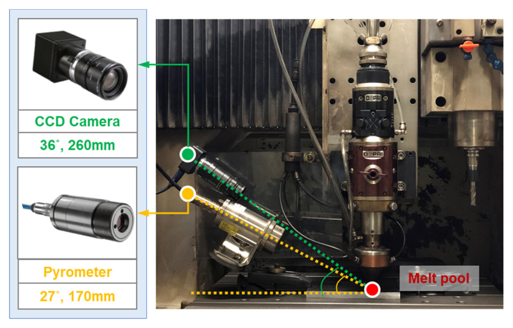
For DED experiments, gas-atomized stainless steel 316L metal powder (Metcoclad 316L, Oerlikon Metco) with a spherical shape and an average particle size between 44 m and 106 m was utilized. In addition, the substrate is made of carbon steel (AISI 1045) and its size is 100 × 150 × 10 mm. The DED experiments were conducted in the DED testbed, and its photo is given in Fig. 1.

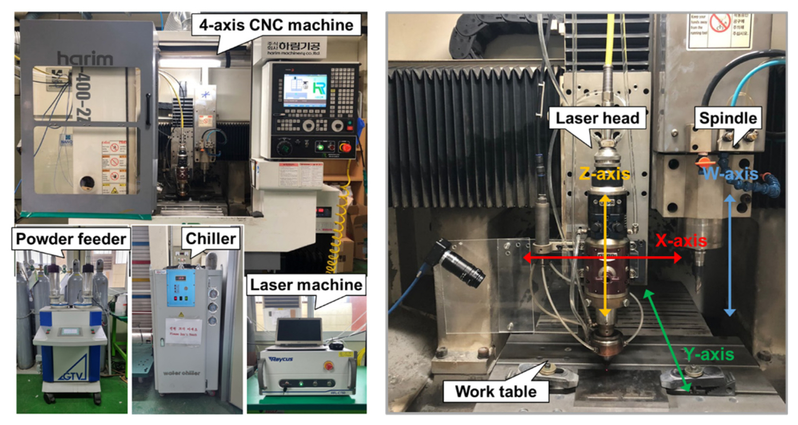
The chemical comopositions of the powder and substrate are detailed in Table 1, and Table 2 shows the experimental conditions, which was considered in the previous study of the authors’ research group [12]. As depicted in Fig. 2, the deposition part had the rectagular configuration whose size was 20 × 15 mm with a single layer.

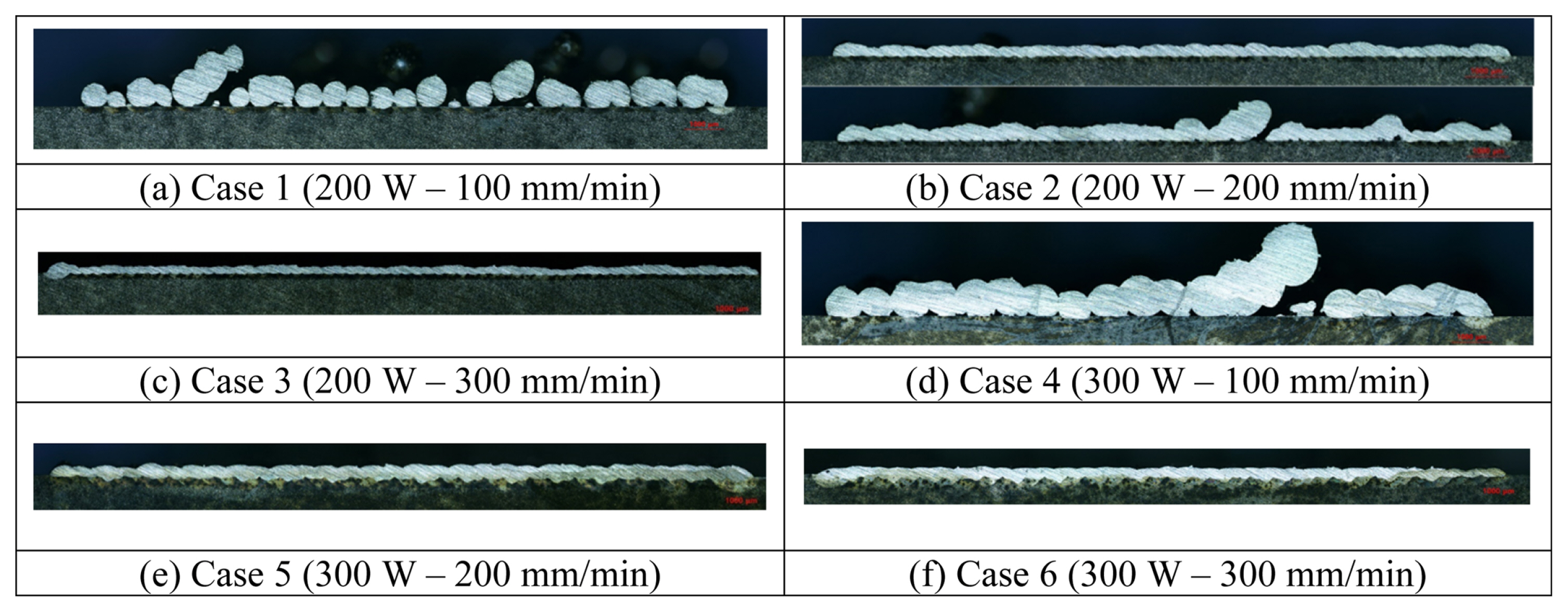
Among the as-deposited parts given in [12], both those with a defect of melting balls and those in a normal state were considered. Fig. 3 depicts images of cross-sectional views of the as-deposited parts. Cases 1, 2, and 3 represent the state of a melting ball, while cases 4, 5, and 6 represent normal states. When the energy density is low and there is an excess of powders, the melting balls can be created.

2.2 Image pre-processing

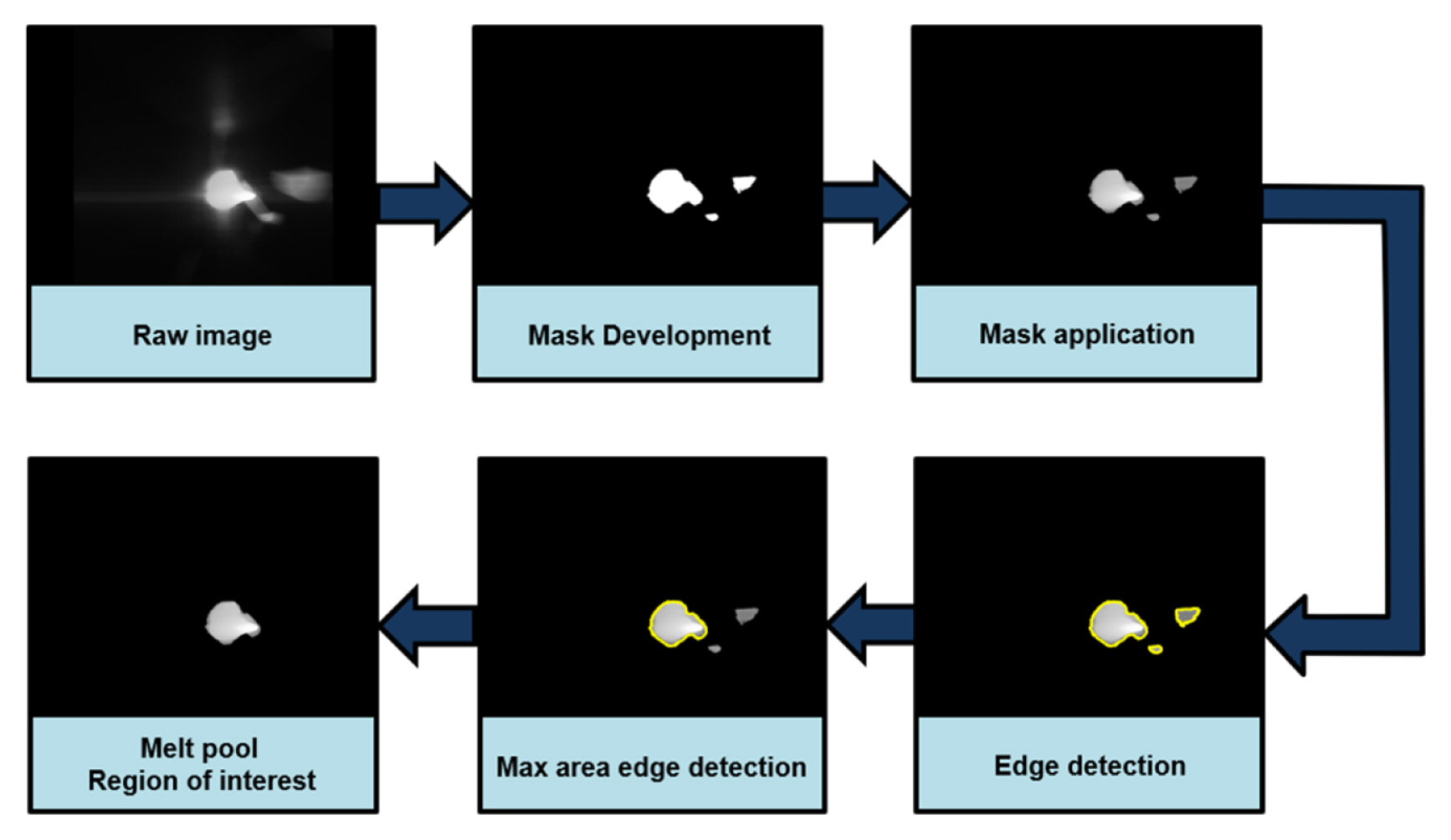
In this research, the off-axial melt-pool monitoring setup was installed by positioning the CCD camera (CM3-U3–13Y3M, FLIR) at an angle of 36 degrees and 260 mm from the melt pool, as can be seen in Fig. 4. Even though a near-infrared filter was attached to the CCD camera, noisy pixels caused by spatter and scattered powders during the DED process should be appropriately removed. Thus, as depicted in Fig. 5, OpenCV-based image pre-processing steps were carried out to eliminate these noises and extract region of interest (ROI) images of the melt pool.

During the image preprocessing, the CCD camera captured images of the melt pool at 30 frames per second, and a mask was produced from the raw image by applying a thresholding algorithm. The mask was applied to the images of the melt-pool, and those with pixel values below the threshold limit were removed. Upon the application of contour extraction, a large area was selected for the melt-pool and a small area was selected for noises, spatters, and scattered powders via maximum area edge detection.

2.3 Degree of Irregularity

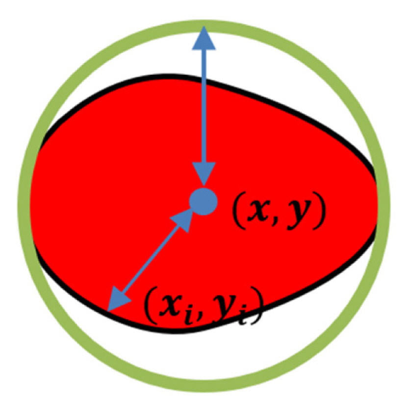
In this study, the degree of irregularity (DOI) is proposed as a new index for characterizing the melt-pool for diagnosing the DED quality. DOI computes the ratio of the distance from the circumference’s center point to the node of the melt pool’s boundary to the circumferential radius of the melt pool. The formula calculating DOI is given by the following equation.

As shown in Fig. 6, (x_i, y_i) is the location of the melt pool boundary node point, and (x, y) is the center of the circumcircle. DOI is the sum of the distance between the circumcircle’s center point and each node’s point, divided by the circumcircle’s radius, divided by the total number of nodes. It would be suitable for monitoring the continuous DED process if DOI could indicate the degree to which the melt pool is non-uniform based on the ratio between the circumcircle and the melt pool.

3. DED Defect Diagnosis

The DOI time series data from melt-pool were utilized to develop an AI-based DED defect diagnosis model. In particular, the short-time Fourier transform (STFT) and Hilbert-Huang transform (HHT) methods have been applied, and the diagnosis results were compared.

3.1 STFT Method

STFT utilizes a fixed-length window function to execute a Fourier transform on short time segments in order to obtain the local spectrum of each segment. The set of transformed local spectra by STFT is appropriate for Convolutional Neural Networks (CNN) because it provides time-domain and frequency-domain spectral information [13].

The basic calculation formula of STFT is given as follows:

(3)

STFT{x(t)}(τ,ω)≡X(τ,ω)=∫-∞∞x(t)ω(t-τ)e-iωtdt

where ω(t−τ)) is the shifted window, x(t) is the time-domain signal, τ is the time index and t means the time, and ω means the frequency. The length of the window function determines the spectrum’s time and frequency resolution. Shorter window lengths enhance time domain resolution with STFT but decrease frequency domain resolution. In contrast, a wider window function improves frequency domain resolution but degrades time-domain resolution.

3.2 HHT Method

Huang proposed the Hilbert–Huang Transform (HHT), which combines the Empirical Mode Decomposition (EMD) and Hilbert Spectral Analysis (HSA) approaches. [14].

(1) Empirical Mode Decomposition (EMD) and Ensemble Empirical Mode Decomposition (EEMD)

The EMD separates the nonlinear and nonstationary multicomponent signal into simplified periodic modes known as Intrinsic Mode Functions (IMF). Through the process of sifting, EMD decomposes the original signal into IMFs one by one until the residue is monotonous.

Step 1: Identify the extrema (local minima Lm_i, i = 1, 2, … and local maxima Lx_i, i = 1, 2, …) using input signal x[n]
Step 2: Obtain U_e[n] and L_e[n], which are upper and lower envelopes respectively, using cubic interpolation.
Step 3: Calculate the local mean value of the upper and lower envelopes.
Step 4: Compute d₁[n] = x[n]−M_e[n]. If d₁[n] satisfies the condition of IMF, d₁[n] = IMF₁[n], else reiterate steps 1 – 4 using d₁[n] instead of x[n].
Step 5: After obtaining IMF₁[n], calculate the residue R_L[n] = x[n] − IMF₁[n]. If this residue has more than a zero-cross, return to step 1 and calculate new IMF.

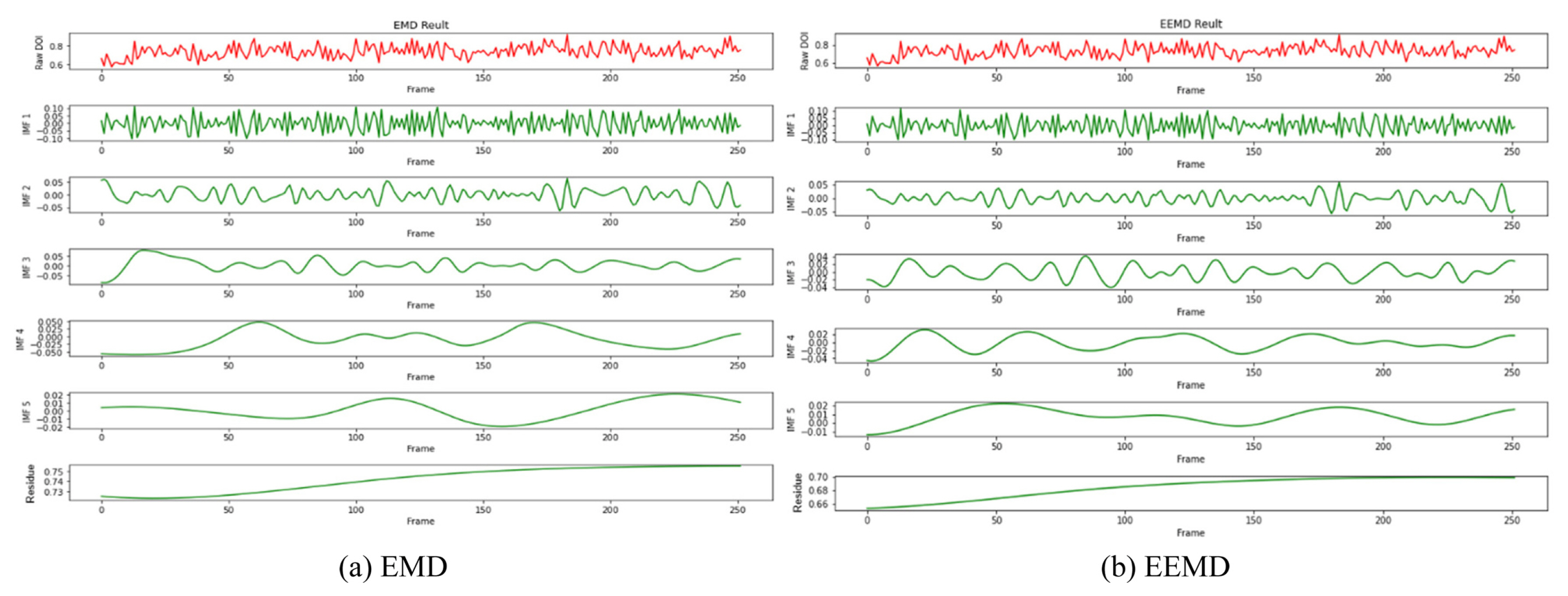
However, mode mixing problems can arise when the EMD method is applied practically. The definition of the mode mixing problem is that signals of widely different scales or indistinguishable scales remain in different IMF components, causing severe noise in the time-frequency distribution and destabilizing the physical meaning of independent IMF. Therefore, Wu and Huang proposed a noise-assisted EMD algorithm called ensemble empirical mode decomposition (EEMD), and it can automatically eliminate the mode mixing problem [15]. In the EEMD process, the chunks of signals of different scales can be automatically transformed into the proper scales of reference established by adding white noise to the data. Fig. 7 shows the decomposed signals from EMD and EEMD, which include IMFs extracted from the DOI time series data for a 200 W laser and 100 mm/min scanning speed. Fig. 7(b), in comparison to Fig. 7(a), demonstrates that EEMD effectively eliminates mode mixing in EMD.

(2) Hilbert Spectral Analysis (HSA)

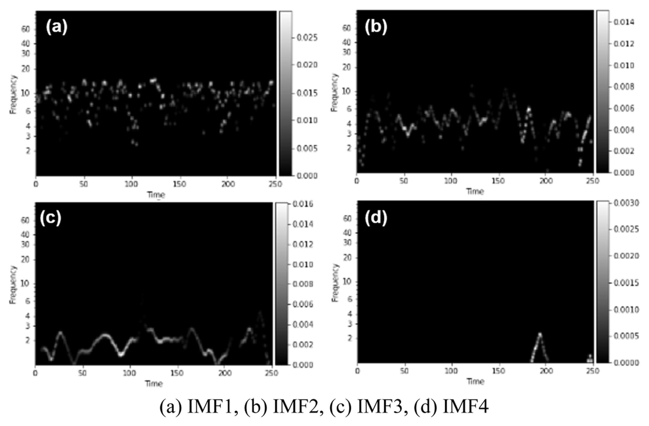
The Hilbert Spectrum (HS) is a time-frequency signal description. Unlike STFT, however, HS does not utilize a fixed resolution window length. It follows the process of the time-frequency basis in the original signal adaptively and can provide more comprehensive information at varying time-frequency scales. After calculating the IMFs, the instantaneous amplitude and phase of each IMF can be determined. The Hilbert spectrum H(ω, t) can be plotted as the instantaneous amplitude as a function of time at the instantaneous frequency.

A major difference between STFT and HS is that the instantaneous function of HS retains the frequency’s dynamic information, enabling minute but sparse explanations. In other words, only HS retains information regarding how the frequency changes in the original time series. Fig. 8 shows the HS samples of IMFs. When observing them, the HS of IMF 1 and IMF 2 reflect more dynamic frequency behavior of the signals, while that of IMF 4 represent low frequency behavior.

3.3 2D-Convolutional Neural Network (CNN) Based Defect Diagnosis

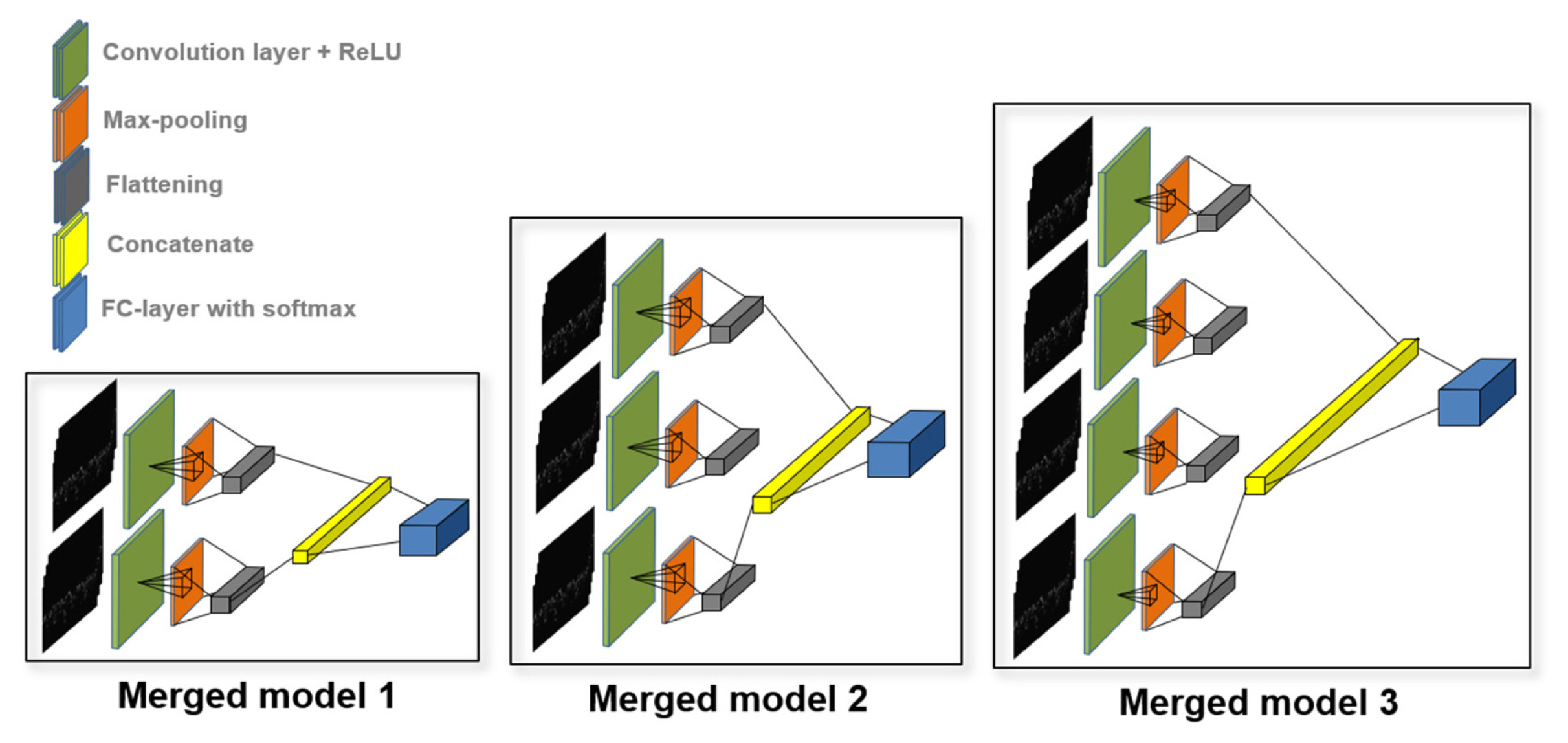
When establishing 2D-CNN models with HS of DOI time series data, various combinations of IMFs were considered. As can be seen in Table 3, the merged model 1 is comprised of two distinct IMF data, the merged model 2 is comprised of three distinct IMF data, and the merged model 3 is comprised of four distinct IMF data. Fig. 9 illustrates schematics of the 2D-CNN architectures of each merged model.

The grid search method was applied to obtain best merged model and optimal hyperparameters for the 2D-CNN model. After the grid search process with the datasets of 37 replications for 6 cases, the (1+2+3) IMF combination was selected as the best merged model, and the optimal hyperparameters are summarized in Table 4.

In order to improve the performance of deep learning methods, the K-fold cross-validation approach was applied. In this research, 4-fold cross-validation was applied, and the average validation accuracy for diagnosing the normal and balling states was 85.68%. Finally, a total of 12 replications of six cases were prepared for testing the developed model based on HHT. The testing accuracies for the normal and balling states were 76.65% and 96.92%, respectively. While the model based on conventional STFT showed testing accuracies of 65.36% and 80.00%, respectively. Therefore, it was demonstrated that the HHT-based 2D-CNN model had superior performance to the STFT-based model.

4 Conclusion

This paper proposes a new feature index — the degree of irregularity (DOI) — that can be used for defect diagnosis during the DED process when monitoring the melt pool. In addition, time series data of the DOI during the DED process was processed by introducing the Hilbert-Huang transform (HHT) for input to the 2D-CNN-based diagnosis model. In the HHT-based data processing phase, ensemble empirical mode decomposition (EEMD), which decomposes original DOI data into multiple frequency domains, was used to avoid mode mixing. Using grid search optimization and K-fold cross-validation techniques the optimal DED defect diagnosis model has been developed. The final testing accuracies for normal and balling states were 76.65% and 96.92%, respectively, which is approximately 10 to 15% higher than the conventional STFT-based diagnosis model. Consequently, it was demonstrated that the HHT-based data processing with EEMD of time-series data of the proposed DOI improved the accuracy of defect diagnosis for the DED process through melt-pool monitoring.

Acknowledgment

This research was supported by the National Research Foundation of Korea (NRF) grant (NRF-2022R1A2C3012900), funded by the Korea government (MSIT).

Fig. 1

Photo of the DED experimental testbed

Fig. 2

Schematic of the DED path and photo of the as-deposited part [12] (Adapted from Ref. 12 on the basis of OA)

Fig. 3

Cross-sectional images of as-deposited parts [12] (Adapted from Ref. 12 on the basis of OA)

Fig. 4

Photo of the melt-pool monitoring system [12] (Adapted from Ref. 12 on the basis of OA)

Fig. 5

Schematic diagrams of image pre-processing steps

Fig. 6

Schematic for calculating the degree of irregularity (DOI)

Fig. 7

Samples of the decomposed signals from EMD and EEMD

Fig. 8

Sample results of HS of DOI time series data

Fig. 9

Schematic diagrams of 2D CNN architectures with various merged models

Table 1

Chemical composition of powder and substrate

Content	Fe	Ni	Cr	Si	Mn	C	Others
SAE 316L	Bal.	12	17	2.5	1.0	0.03	≤ 0.5
AISI 1045	Bal.	-	-	-	0.7	0.45	-

Table 2

Experimental conditions [12] (Adapted from Ref. 12 on the basis of OA)

Laser power (W)	200, 300, 400, 500, 600
Scanning speed (mm/min)	100, 200, 300
Mass flow rate of powder (g/min)	10
Delivery gas flow rate (L/min)	14
Shielding gas flow rate (L/min)	12
Substrate	AISI 1045
Metal powder	SAE 316L
Overlap (%)	35
Stand-off distance (mm)	10
Size of the substrate (mm)	100 × 150 × 10

Table 3

Various merged models with different combinations of IMFs

Merged model 1	Merged model 2	Merged model 3
IMF 1+2	IMF 1+2+3	IMF 1+2+3+4
IMF 1+3	IMF 1+2+4
IMF 1+4	IMF 2+3+4
IMF 2+3
IMF 2+4
IMF 3+4

Table 4

The best merged model and optimal hyperparameters after grid search

Combination of IMFs	Kernel size	Dense neurons	Learning rate	Drop out	Accuracy
IMF 1+2+3	4	400	0.0001	0.6	0.919081

Reference

1. ISO/ASTM 52900(en). (2018). Additive manufacturing — General principles — Terminology https://www.iso.org/obp/ui/#iso:std:iso-astm:52900:dis:ed-2:v1:en)

2. Xiao, X., Lu, C., Fu, Y., Ye, X. & Song, L. (2021). Progress on experimental study of melt pool flow dynamics in laser material processing. Liquid Metals.

3. Zheng, L., Zhang, Q., Cao, H., Wu, W., Ma, H., Ding, X., Yang, J., Duan, X. & Fan, S. (2019). Melt pool boundary extraction and its width prediction from infrared images in selective laser melting. Materials & Design, 183, 108110.

4. Akbari, M., & Kovacevic, R. (2018). An investigation on mechanical and microstructural properties of 316LSi parts fabricated by a robotized laser/wire direct metal deposition system. Additive Manufacturing, 23, 487–497.

5. Manvatkar, V., De, A. & DebRoy, T. (2015). Spatial variation of melt pool geometry, peak temperature and solidification parameters during laser assisted additive manufacturing process. Materials Science and Technology, 31(8), 924–930.

6. Tang, Z.-J., Liu, W.-W., Wang, Y.-W., Saleheen, K.M., Liu, Z.-C., Peng, S.-T., Zhang, Z. & Zhang, H.-C. (2020). A review on in situ monitoring technology for directed energy deposition of metals. The International Journal of Advanced Manufacturing Technology, 108, 3437–3463.

7. Khanzadeh, M., Chowdhury, S.Bian, L. & Tschopp, M.A. (2017). A methodology for predicting porosity from thermal imaging of melt pools in additive manufacturing thin wall sections. In: Proceedings of the International Manufacturing Science and Engineering Conference; V002T001A044.

8. Mi, J., Zhang, Y., Li, H., Shen, S., Yang, Y., Song, C., Zhou, X., Duan, Y., Lu, J. & Mai, H. (2021). In-situ monitoring laser based directed energy deposition process with deep convolutional neural network. Journal of Intelligent Manufacturing (pp. 1–11.

9. Zhang, B., Liu, S. & Shin, Y.C. (2019). In-Process monitoring of porosity during laser additive manufacturing process. Additive Manufacturing, 28, 497–505.

10. Li, J., Cao, L., Xu, J., Wang, S. & Zhou, Q. (2022). In situ porosity intelligent classification of selective laser melting based on coaxial monitoring and image processing. Measurement, 187, 110232.

11. Zhang, Y., Soon, H.G., Ye, D., Fuh, J.Y.H. & Zhu, K. (2019). Powder-bed fusion process monitoring by machine vision with hybrid convolutional neural networks. IEEE Transactions on Industrial Informatics, 16(9), 5769–5779.

12. Lee, J., (2021). Development of multiple defect diagnosis algorithm for directed energy deposition process based on artificial intelligence. Master Thesis. Sungkyunkwan University.

13. Allen, J., (1977). Short term spectral analysis, synthesis, and modification by discrete Fourier transform. IEEE Transactions on Acoustics, Speech, and Signal Processing, 25(3), 235–238.

14. Huang, N.E., Shen, Z.Long, S.R.Wu, M.C.Shih, H.H.Zheng, Q.Yen, N.-C.Tung, C.C. & Liu, H.H. (1998). The empirical mode decomposition and the Hilbert spectrum for nonlinear and non-stationary time series analysis. In: Proceedings of the Royal Society of London. Series A: Mathematical, Physical and Engineering Sciences; 454(1971)pp 903–995.

15. Wu, Z., & Huang, N.E. (2009). Ensemble empirical mode decomposition: A noise-assisted data analysis method. Advances in Adaptive Data Analysis, 1(01), 1–41.

Biography

Jun Ho Kong received his B.S. degree in the School of Mechanical Engineering from Dalian University of Technology, China, in 2019, and his M.S. degree in the Department of Mechanical Engineering at Sungkyunkwan University, Korea, in 2022. His research interests include metal 3D printing, prognostics and health management (PHM) and artificial intelligence.

Biography

Sang Won Lee received his B.S. and M.S. degrees in the Department of Mechanical Design and Production Engineering from Seoul National University, South Korea, in 1995 and 1997. He received Ph.D. in the department of Mechanical Engineering from University of Michigan, Ann Arbor, MI, USA, in 2004. Dr. Lee joined the School of Mechanical Engineering at Sungkyunkwan University in 2006, and is currently a Professor. His research interests include smart factory, prognostics and health management (PHM), cyber-physical system (CPS), environmentally-friendly mechanical machining, additive manufacturing, and data-driven design.