Cho, Seo, Lee, Choi, and Choi: A Rapid Learning Model based on Selected Frequency Range Spectral Subtraction for the Data-Driven Fault Diagnosis of Manufacturing Systems
Abstract
Limited amount of training dataset is often a critical problem in developing a diagnosis model or computational intelligence of mechanical failures. In this paper, we propose a Selected Frequency Range Critical Information Map (SFCIM)-based data-driven diagnosis method for detecting mechanical system failure with a relatively small amount of available dataset. The algorithm determines whether there is a failure with reference to normal condition signals using the spectral subtraction method. In this process, time-domain synchronization and time-frequency representation are applied. In addition, the dominant frequency range is selected based on FisherŌĆÖs scores for the more efficient calculation. We designed this algorithm to provide users with time-frequency domain information about system failure through SFCIM instead of the only simple decision of diagnosis. The usefulness of our method has been checked with the following problems of the small amount of available dataset: diagnoses of (1) the IMS bearing faults, (2) input gear faults of a manipulator driving system, and (3) a driving system of an industrial robot by load current signals. From these case studies, we also confirmed that the proposed method was practical and useful for fault diagnosis regardless of signal types, such as stationary, non-stationary, accelerometer-based vibration, or current signal.
Keywords: Selected frequency range critical information map (SFCIM) ┬Ę Fault diagnosis model ┬Ę Data-driven approach ┬Ę Spectral subtraction ┬Ę Frequency range selection ┬Ę Time-frequency representation
1 Introduction
Sudden failures of mechanical systems may cause catastrophic disasters with losses of invaluable human lives and severely disturb production processes, including massive time and financial losses. Condition-based maintenance (CBM) has been proposed to reduce system downtime and increase maintenance efficiency by monitoring real-time signals and predicting the remaining useful life of the system. The real-time monitoring of mechanical systems in CBM employs various types of signals, such as accelerometer-based vibration [ 1, 2], current [ 3, 4], and torque [ 5]. A vibration signal measured using an accelerometer or an acoustic emission sensor is the most common signal used to diagnose a system fault. Vibration signals acquired at a high sampling rate are useful for the fault diagnosis of a rotating machine with high-frequency characteristics such as the mesh frequency of a gearbox and the bearing fault frequency [ 6, 7]. Fault diagnosis may be categorized into model-based, signal-based, and knowledge-based approaches [ 8, 9]. In the model-based and signal-based approaches, diagnosis models are required to be developed based on professional signal-processing knowledge or detailed information about the system. Therefore, it is difficult for engineers to apply these approaches to a complex system about which only limited knowledge is available. For example, Li et al. [ 10] transformed vibration signals to the frequency domain to monitor bearing conditions using the characteristic fault frequency calculated from their bearing structure. In addition, Kong et al. [ 11] proposed a fault diagnosis method for a planetary ring gear based on the mesh frequency of the gear structure. These approaches mainly apply to the cases where signals are stationary but cannot to the non-stationary signal cases. To overcome these challenges, researchers employed a knowledge-based approach, called a data-driven approach.
In this approach, a failure diagnosis model is developed using machine learning techniques using big data. This approach is applicable to a system in which expert knowledge is limited. In the data-driven approach, we tend to employ signal processing techniques since it is difficult to extract useful information from the raw signals. Chen et al. [ 12] proposed a bearing fault diagnosis model that applied a one-dimensional (1D) convolutional neural network (CNN) model to the vibration signal. Zhang et al. [ 13] converted the acquired raw vibration signal into a timeŌĆōfrequency domain spectrogram using the short-time Fourier transform (STFT). They diagnosed bearing defects using a deep two-dimensional (2D) CNN model. However, the data-driven approach often requires a large amount of data for developers to train their models. It is usually challenging to acquire enough training data to develop artificial intelligence with a reasonable level of accuracy. This difficulty is even more significant in monitoring actual manufacturing processes because of the high cost in the acquiring qualified data and very limited amount of failure state data. While overcoming the challenges of the data-driven approach, the goal in this work is developing a high-accuracy data-driven diagnosis method applicable to the problems of (1) a small amount of training data set, (2) non-stationary signals, and (3) current signals, (4) providing user-friendly diagnosis information to users.
This paper is organized as follows. Section 2 presents a description of the approach proposed in this study. Section 3 presents the performance of the proposed method with various case studies of different mechanical systems with various types of measurements for the diagnosis, such as non-stationary vibration signals or current signals. In Section 4, we compare the performance of our approach with that of other data-driven methods. Finally, we summarize the results of this study in Section 5.
2 SFCIM-based Fault Diagnosis Method
The Selected Frequency Range Critical Information Map (SFCIM)-based fault diagnosis algorithm proposed in this study employs spectral subtraction of the signals acquired in the normal or faulty condition. A frequency band that has a dominant effect on fault diagnosis is selected and analyzed during the process. The area where the difference commonly occurs between the subtracted spectrograms of the normal and faulty conditions is found through an optimization process. We call this area an outstanding window (OW) and the optimization process as training. The algorithm investigates whether the OWs of a newly observed signal are similar to those of normal or faulty condition. The overall process is shown in Fig. 1 and described step-by-step as follows.
Step 1. The time-domain synchronization of the raw signal for training is completed through cross-correlation in the time domain. Step 2. Using wavelet packet decomposition (WPD), the normal and faulty signals for training are converted into time-frequency domain spectrograms. Step 3. Normal-reference (N-R) and abnormal-reference (A-R) spectrograms for training are obtained by spectral subtraction of a reference spectrogram, which we usually set from one of the normal signals. Step 4. Three statistical features are extracted from the coefficients of each frequency level of the N-R and A-R spectrograms. Important frequency ranges for diagnosis are ranked using FisherŌĆÖs scores. Step 5. Among the user-defined variables, important feature values are selected according to the window selection ratio (WSR). The effective band is the frequency band in which all three features are selected as important areas. Moreover, one band each of higher and lower bands are additionally selected for conservative selection. A further detail WPD analysis in a selected frequency range with a user defined magnification ratio (MR) may be optionally necessary. Step 6. Through an optimization process (i.e., training), we determine the OWs in a spectrogram, which areas the areas where the difference between the N-R and A-R spectrograms is consistently observed. We call the spectrogram map with the OWs a Selected Frequency Range Critical Information Map (SFCIM). Step 7. A mechanical system is classified as a normal or faulty condition by the number of OWs. If those are closer to the faulty condition, we may determine the system is in the faulty condition.
2.1 Time-Domain Data Synchronization
Generally, a time delay occurs between the collected raw data samples. Eliminating the time delay, time-domain synchronization using cross-correlation is required. This synchronization process reduces the time-band error on the subtracted spectrogram, making it possible to compare the difference between normal and faulty conditions without the time delay.
Cross-correlation is often used to synchronize time-series signals with different time lags. The correlation between two signals in the time domain is calculated as follows [ 14]: where f is the signal to be synchronized, g denotes the reference signal for obtaining the time delay, and ╬┤ denotes the time delay between the two signals. We define ╬┤max as the time point that shows the highest cross-correlation value and obtain the synchronized signal by applying the ╬┤max value to the raw signal f.
2.2 Time Frequency Representation and Spectral Subtraction Process
A signal spectrogram is important for a user to recognize the fault area in the timeŌĆōfrequency domain, which is the beginning process of developing SFCIM. Time-Frequency Representation (TFR) that converts the acquired and synchronized raw signal into a timeŌĆōfrequency domain includes the following transformation methods (1) STFT, (2) discrete wavelet transforms (DWT), and (3) WPD.
In the STFT, a user should define the window size in the time and frequency domains. Depending on this user definition, the resolution of the time and frequency bands changes, to which signal analysis results are very sensitive [ 15]. Verstraete et al. [ 16] found that a CNN-based learning model is not highly reliable when it is trained using STFT-based 2D spectrogram images. On the other hand, WT solves the window-size issue by introducing a window size that varies in the time and frequency domains. Furthermore, in DWT, different window sizes are applied for each frequency band. The resolution of the time band decreases in the lower frequency band, and that of the frequency band decreases in the higher frequency band. The WPD technique maintains the same high resolution in both low- and high-frequency bands. In this study, we employ the WPD among the three techniques to develop the SFCIM. The WPD starts with a decomposition process based on the kernel function in Eq. (3): where j is a scale factor at the corresponding decomposition level; k is the shifting parameter (i.e., translation along the time axis); and n is a modulation or oscillation parameter. The first and second wavelet packet functions become scaling and mother wavelet functions, respectively, and the general formula is defined as follows:
where h(k) and g(k) are quadrature mirror filters and orthogonal to each other. Therefore, the wavelet packet coefficients expressed by variables j, n, and k are as follows:
where f( t) is the signal to be decomposed. The WPD is used to generate the SFCIM. Details of the WPD may be referred in Ref. 17. In developing the SFCIM, a reference signal and spectral subtraction are performed to compare the signal under normal and abnormal conditions. We may draw an analogy between this subtraction process and filtering out noises from speech signals.
The noise-filtered signal spectrogram with spectral subtraction is as follows:
where Sv( Žē) is a spectrogram of the signal that includes noise, Sn( Žē) and is a spectrogram of a noise signal without a valid voice. Berouti et al. [ 18] obtained the noise-removed signal using Fourier inversion of SvŌĆ▓( Žē). Denda et al. [ 19] presented a spectral subtraction method for a wavelet transform-based spectrogram. Our method uses the following equation: where | X╠é( b,a)| is the wavelet spectrogram of the filtered signal, | ╬│s( b,a)| is the wavelet spectrogram of the raw signal, including noise,
|Nn(b,a)¯| is the wavelet spectrogram of the noise, α is a reduction factor indicating the degree of noise removal, and a and b are the time-domain position and scale parameters of the wavelet filter, respectively. Bouchikhi et al. [ 20] applied the noise-reduction concept to bearing fault diagnosis. In this study, we perform spectral subtraction based on Eq. (8). The reference signal is set by randomly selecting one among the normal signals. Our fault diagnosis algorithm prepares two groups of training spectrograms, which are N-R spectrograms (i.e., the subtracted wavelet spectrograms between those of the normal and reference signal) and A-R spectrograms (i.e., the subtracted wavelet spectrogram between those of the signal collected in the failure condition and the reference signal). The case studies in Section 3 describe this process in detail.
2.3 Dominant Frequency Range Selection and Additional Detailed Analysis Process
The original purpose of the feature selection is to eliminate unnecessary features in the artificial intelligence development process and find the optimized feature subset. Through this process, it is possible to prevent overfitting and develop an effective model with increased generalizability. This study uses the method of ranking features based on the Fisher score corresponding to the filter method [ 21]. The Fisher score filter method gives a higher rank as the distance between clusters of data increases, and each cluster is densely distributed. The main concept of finding OW through the optimization process presented later is to find a constant and large difference in the signal spectrogram. In this process, we intend to make the optimization process more efficient by applying the characteristics of FisherŌĆÖs score to select the frequency level at which OW will occur. The score of each feature used to rank the features is as Eq. (9), where j means the class number corresponding to the classification target of the model, i is the sequence number of the feature, nj is the number of data samples of the jth class, ╬╝i is the overall average value of the ith feature, ╬╝i,j is the mean value of the jth class cluster of the ith feature, and Žāi,j is the internal variance value of the jth class cluster of the ith feature. The larger the Fisher score ( fi) of each feature, the greater the density of the features in the cluster for each class.
FisherŌĆÖs score-based feature selection is introduced to select a frequency range that is effective for fault diagnosis, as shown in Fig. 2. This range selection process defines the useful area for fault diagnosis in the signal spectrogram and reduces the computation time for searching OWs in the following optimization process. For selecting the highly sensitive frequency range to system conditions to monitor, the SFCIM uses three statistical features: the root mean square (RMS), the absolute mean, and the maximum values of each frequency band. The mathematical definitions of RMS and absolute mean are listed in Eqs. (10) and (11) respectively, where n is the number of coefficients in each frequency range, and ci is the ith coefficient value. The frequency level selection process preceding the optimization process selects a range with a big difference between N-R and A-R at each frequency level of the learning data. In other words, frequency levels that show a constant and significant difference that reflects the characteristics of the high FisherŌĆÖs score features are selected. In Fig. 2, one frequency level is shown as an example. Three statistical features of the coefficient values within the frequency level indicate the difference between N-R and A-R. In this step, we could select the section where the high-ranked features are intensively distributed. The frequency range selection proceeds according to Steps 4 to 5 described in Section 2, and an additional optional step according to the userŌĆÖs optional choice. To explain the two user-defined variables, the user defines the window selection ratio (WSR) as a real number between zero and one. As this value decreases, fewer frequency bands are selected, and as this value increases, more frequency bands are selected.
According to the userŌĆÖs selection, the magnification ratio (MR), is defined as a positive integer, and additional WPD is performed in MR steps and decomposed into 2MR frequency levels. The user experimentally sets the WSR, and MR values based on the basic characteristics of the diagnosis object (i.e., AC current frequency or vibration characteristics of the system). We recommend that the users set the WSR value by starting with a value close to one and set the MR value when detailed analysis is required according to the userŌĆÖs needs.
2.4 Optimization Process for SFCIM
The optimization process corresponds to Step 6 described in Section 2 and the problem formulation of the optimization process is shown in Fig. 3. The objective function in this optimization is to maximize the normalized area of the OWs on the entire map. The reference map is a randomly selected sample from training data with the normal condition. Nn and Na are training datasets of each normal and abnormal condition, respectively. Df is the number of divisions along the frequency band. Ls is the signal length used for model learning (multiplication of time and sampling rate). Nn-r,ij means the number of OWs on the (i, j) window among training data in a normal condition, in and Na-r,ij is the number of OW occurrences on the window among training data in an abnormal condition.
The three design variables to find in this process is illustrated in detail in Fig. 4. The first design variable, x1, is the number of divisions in the time band of the spectrogram. As an example, in Fig. 4, as the value of x1 increases, the time domain division on the spectrogram increases and create more detailed windows. The second one, x2, is the threshold of the difference value between the wavelet coefficients inside the window divided in the timeŌĆōfrequency band. The third one, x3, is a threshold number for determining whether each window is outstanding based on the number of values that exceed the x2 threshold. x2 and x3 are used as thresholds to determine whether each window is outstanding. For example, in Fig. 4, if x2 is 0.4 and x3 is 10, the window becomes OW; if x2 is 0.4 and x3 is 20, it cannot be OW. The Rc value is a criterion value for determining the OW; as it decreases, it tends to be more tolerant of noise inside the training data. For a conservative fault diagnosis, the Cp value is designated as one or more, to reduce the occurrence of OWs in the data under normal conditions.
3 Application to Case Studies
3.1 Center of Intelligent Maintenance Systems Bearing Data
The Center of Intelligent Maintenance Systems (IMS) dataset has often been used as the reference for validating methods and algorithms in many fault diagnosis and prediction studies [ 22]. This vibration signal dataset was measured using an accelerometer installed in the radial direction of bearings supporting a rotating shaft. The shaft was rotating at a constant speed of 2,000 RPM and powered by an AC motor. A spring mechanism in the radial direction of the shaft applied 6000lbs load. The schematic of the data acquisition setup is shown in Fig. 5, in which 20,480 points are measured at every 10 minutes at a sampling rate of 20 kHz. In this case study, we validate the performance of the SFCIM-based fault diagnosis model using the accelerometer signal of the third bearing of the first dataset among the four experimental datasets. As shown in Figure 6, we assume that the bearing signals obtained at the initial condition as normal signals and those at the endpoint of the experiment (i.e., before the failure occurred) as abnormal signals. For data segmentation, we defined the training set of 60 samples close to each condition and the remaining 200 samples as the validation set of the model. The segmentation of the training and validation sets is shown in Fig. 6. We apply an SFCIM-based diagnosis model to the IMS dataset as the steps presented in Section 2. The proposed method has a concept of finding differences according to failures compared to normal conditions. Therefore, in this case study, the reference spectrogram used the data in the state closest to the normal condition among the training data. The Normal-Reference (N-R) and Abnormal-Reference (A-R) subtracted spectrograms obtained with finishing Step 3 of the algorithm are shown in Fig. 7. From Step 4 to 5, the frequency range selection process selects the critical frequency range for the fault diagnosis. The RMS, absolute mean, and maximum values are obtained as statistical features for each frequency level. After combining the extracted statistical features with labels corresponding to the normal and faulty conditions, the process selects the upper-ranked feature value using the Fisher score. With the ranked features, we select the frequency level in which all three statistical features are highly ranked including one level above and below for conservative selection. The WSR value was defined as 0.67, and the selected frequency range was from level 1 to level 2, and from level 6 to level 18, among the 32 wavelet decomposition levels. Only the data of the selected frequency levels were used as input in the optimization process to find the OWs. Using the input of the frequency band data selected through the above process, Table 1 shows the optimized design variables to generate the SFCIM obtained by the optimization process corresponding to Step 6 of Section 2.
Fig. 8 shows the results of determining the OWs using the optimized parameters.
To explain the previous classification results, we would like to discuss the one example window determined as OW. According to the optimization result value of Table 1, the window corresponding to the 1st time interval section of the frequency level 7 of SFCIM shown in Fig. 9 is OW. Figs 9(a) and 9(b) show the coefficients in the corresponding window in the N-R and A-R subtracted spectrogram, respectively. In the N-R subtracted spectrogram of Fig. 9(a), only two of the 128 coefficient values exceed the optimized x2 threshold value (0.1972). However, in the case of the A-R subtracted spectrogram shown in Fig. 9(b), more than ten coefficients are greater than the x2 threshold. When we apply the optimized x 3 variable value to the result, we can confirm that the corresponding window is OW, and through this process, all windows in the SFCIM are determined. Through this process, the model can classify the fault using the number defined OW, and we discuss the validation results below. The SFCIM-based diagnosis model classifies the bearing condition based on the number of OWs. As a result of the validation using 200 new observations (i.e., unused data for training) from each case, as shown in Fig. 10, we can confirm that the result shows a clean separation. Table 2 displays the classification results in a confusion matrix, showing 100% accuracy when validating the algorithm with test data not included in the training process.
3.2 Fault Detection of the Industrial Robot Input Gear
A second case study is the failure diagnosis of a 6-axis industrial robot using vibration signals. An industrial robot is a complex mechanical system that combines various mechanical devices, such as gears, bearings, and belts. Unlike the bearing case, robots move inconsistently. Thus, the acquired signals from those are often non-stationary. In this case study, the diagnosis target is a pitting fault occurring on the surface of the input gear inside the robot driving system [ 23]. The three different defects are classified into normal condition, soft, and hard pitting condition. Details of the experimental setup are presented in Figure 11. The industrial robot used in the experiments for data collection is model HS-180 by Hyundai robotics normally used in a spotwelding line [ 24]. A PCB Piezotronics model 353B03 accelerometer is used. All data were acquired at a sampling rate of 12.8 kHz using an NI 9232 data acquisition (DAQ) module for 16.6 second. An accelerometer is attached in the radial direction of the second joint of the robot. Three hundred samples are collected under each condition. The training and validation data are randomly grouped, and the validation data are not used in the training process. The diagnosis process of this case study proceeds in two stages, as shown in Fig. 12. In the first stage, we classify the normal and abnormal (including soft and hard pitting). In the following second stage, the two abnormal states are further classified as soft and hard pitting. We randomly selected this case studyŌĆÖs reference spectrum from each stageŌĆÖs relatively less faulty data. We prevented the distortion of the results through repeated experiments. As a result of performing the process from Steps 1 to 3, we obtain subtracted spectrograms between the normal-reference (N-R), soft pitting-reference (S-R) and hard pitting-reference (H-R) as shown in Fig. 13. From Steps 4 to 5, the dominant frequency levels in the first stage are from 4 to 6, 11 to 22, and 27 to 32. The selected levels in the second stage are from 2 to 20 and 31 to 32. The WSR value is set as 0.67 in both the first and second stages. Through the experiment, we collected data for 300 samples in each normal and two-stage failure condition. We randomly selected and used 15 data samples, about 5%, as training data, and the remaining 285 samples were used as validation data. The model development process only contained learning data, and the training process did not include validation data. The subtracted spectrograms become the input data of Step 6, the optimization process for developing SFCIM. Table 3 and 4 list the determined design variables in each classification stage. The SFCIM generated based on the optimized parameters is shown in Fig. 14. Figs. 14(a) and 14(c) show the primary map generated by the result value for each window after the optimization process. The final SFCIMs including selected OWs based on the criteria value ( Rc) are shown in Figures 14(b) and 14(d). The numbers of OWs identified from the unused new observations for validation are plotted in Fig. 15. In the first stage classification result between normal and abnormal (contains both soft and hard pitting data) conditions shown in Fig. 15(a), the number of OWs from the unused validation normal data ranged from zero to nine. On the other hand, the number of OWs from the abnormal ones ranged from 34 to 37, and most of the abnormal data included 37 OWs. In the second classification result between soft and hard pitting shown in Fig. 15(b), the number of OWs from the validation data ranged from zero to 5 and 17 to 20 in soft and hard pitting cases, respectively. In both stage classifications, we may observe a clear difference in the number of OWs from the two condition groups. The classification result in Table 4 shows that the SFCIM-based fault diagnosis model shows an accuracy of 100% between normal condition (NC), soft pitting (SP), and hard pitting (HP). We believe the proposed algorithm can be applied to non-stationary vibration signals and classify multi-stage fault problems. It may also be highlighted that the highly accurate diagnosis model can be achieved with only 5% of the total data samples of each class.
3.3 Grease Level Detection of a Robot based on Current Signals
This case study aims to diagnose grease levels in a driving system using an AC signal loaded on the joint of an industrial robot. Lack of grease in the gearbox may cause the failure of gears and bearings; however, it is difficult to determine the grease level while it is operating. We expect that the failure of a drive system in a robot might be prevented by diagnosing the decrease in the grease level inside.
As shown in Fig. 16, a Yaskawa GP-12 6-axis industrial robot was used in the experiment [ 25]. The payload of this robot is up to 12 kg, and the maximum range in the vertical and horizontal directions was 2,511 mm and 1,440 mm, respectively. The failure mode defined in this case study is a decrease in the grease inside the driving part. The fulfilled amount of grease for the second-axis drive unit is 130 cc, and the recommended maintenance level in the manufacturerŌĆÖs manual is 65 cc [ 26]. We defined the fulfilled grease level (130 cc) as normal, and the grease that decreased to near the maintenance level of 70 cc was defined as faulty. In this case study, we use the current signal, which is easier to collect for engineers than the vibration signal. The current sensors may be installed not on the body of a robot but in between a robot and its controller, which interferes less with the operating robot in a production site. As shown in Figure 16, an FS9L10 current probe manufactured by Fine Trans Tech [ 27] was installed inside the robot controller. The current probe was installed to acquire the current signal applied to the robot driving part one among the three-phase AC power lines from the amplifier module supplying power to the second-axis motor of the robot. The signal was acquired at a sampling frequency of 12.8 kHz and a sampling time of 13.8 s using the NI 9232 DAQ. Two hundred samples of the signals are collected from the robot in both normal (130 cc) and abnormal (70 cc) conditions. 20% of the total data are randomly selected as the training dataset. The remaining samples were used as validation datasets to evaluate the performance of the optimized SFCIM. This case study selected reference data similar to Case Study 2. As a result of performing the process from Steps 1 to 3, we obtain N-R and A-R subtracted spectrograms as shown in Fig. 17. The area showing a significant difference in the A-R and N-R spectrograms is a relatively low-frequency range, reflecting the frequency range characteristics of the AC power applied to the driving motor of the industrial robot. In Steps 4 and 5, the dominant frequency range is from level 1 to level 2, with one level above and below selected for a conservative decision. In this selection, the WSR value is set as 0.16. Unlike Case Studies 1 and 2, the optional step in Step 5 mentioned in Section 2 is required in this case. An additional WPD-based timeŌĆōfrequency decomposition for the selected frequency levels is performed. The MR is defined as 4, and the coefficients of the two selected frequency bands were decomposed into 16 levels.
After the additional timeŌĆōfrequency decomposition, the data samples become input data for Step 6, and an optimized design variable is obtained through the optimization process. Table 5 lists the WSR, and MR values defined, and the final optimized design variables. The optimized SFCIM is shown in Fig. 18. The maximum frequency of the AC signal applied to the drive motor of the second axis used in the experiment is 125 Hz. We observed that OWs on the SFCIM are mainly located within the corresponding frequency levels. The results of diagnosing the condition of the validation dataset based on the OWs of the corresponding SFCIM are presented in Figures 19, and 21 OWs could be seen as the result. The number of OWs of normal data (130 cc) of the validation data ranged from zero to one, and in the abnormal (70 cc) case, the number ranged from 19 to 21. We observed a very clear classification by the number of OWs of normal and abnormal data. As shown in Table 6 as the form of a confusion matrix, validation results in this case study using an AC signal loaded to the driving motor are very promising. We can also confirm that the diagnosis model with high performance can be made with a very small number of training data of 40 for each class, only 20% of the total data.
4 Comparison with Other Data-Driven Methods
This section compares the performance of the SFCIM-based fault diagnosis model proposed in this study with previous data-driven methods. The methods selected for the comparison are two types of CNN using 1D and 2D images of original signals for training and artificial neural network (ANN) using statistical signal features. Ince et al. [ 28] transformed the acquired raw signal to the frequency domain using the fast Fourier transform (FFT) and used it as an input for a 1D CNN model. We apply this technique to the case of the IMS data for comparison. Zhang et al. [ 11] proposed a 2D CNN-based fault diagnosis model using time-frequency domain spectrogram images. We employ the model to compare with the SFCIM-based method. In the case of the statistical feature-based ANN model, seven statistical features from each frequency level decomposed through WPD were extracted. A total of 224 features are extracted from the original signal. Highly relevant features for the diagnosis are selected through a two-step feature selection process. The first step selects the top 50 features using minimum-Redundancy and Maximum-Relevance and (mRMR) [ 29]. The optimum set of features is selected in the second step, the sequential backward selection wrapper method [ 30]. In the data-driven approach, the prediction accuracy decreases as the amount of training data decreases leading to overfitting, which could be a critical problem of the fault diagnosis model. Therefore, we compare the performance of the diagnosis models under the more difficult situation, which uses a small amount of training data. The same process was performed five times in each case for model performance comparison, and the resultsŌĆÖ averages were used for comparison. The model performance is compared based on accuracy, sensitivity, specificity, and precision, which are calculated by the values in a confusion matrix. Details of the mathematical definition are in Ref. [ 31]. In Case Study 1, the results of comparing the model performance of the four methods using 60 data samples (Approximately 23% of total samples as training data) are listed in Table 7. The results show that the SFCIM-based fault diagnosis model can obtain very high accuracy even with small training data. We can see that the specificity and precision values of the SFCIM-based model are high among the performance indicators of the diagnosis result, which means that the number of false positives to diagnose a failure state as normal is small. The false positive situation can lead to a problem by misdiagnosing the failure state. The proposed method can prevent it. One of the advantages of the SFCIM-based fault diagnosis model is high-efficiency in computation. We compared computation time with previously presented Critical Information Map (CIM) based fault diagnosis models through comparative experiments [ 32]. The device used in the experiment used the ASUS FX503VM laptop, consisting of an Intel i7-7700HQ CPU and 24 GB of RAM. In this experiment, we did not use the GPU parallel computation function. The experiment results are shown in Table 8. As shown in the results, the computational time required by the SFCIM is significantly reduced by about 36% comparing with that required by the CIM. The difference of the computational load may be the larger as training data size increases.
5 Conclusions
The SFCIM-based fault diagnosis model shows high diagnostic accuracy even with small training data. In the case studies, we observed excellent results and 100% accuracy in the performance test with a training data set of only a small part of the total data. Especially in Case Study 2, the model performed very well with only 15 samples from the total collected data.
In addition, we believe that the applicability of the SFCIM to the rotational mechanical system is excellent, as demonstrated by the case studies. It was highly applicable to a system with stationary signals (Case Study 1) and a complex system with non-stationary signals (Case Studies 2 and 3).
As shown in Case Study 3, detecting the grease level of the industrial robot driving system using the current signals was highly accurate. We can confirm that the SFCIM performs sufficiently well-monitors mechanical systems using a current signal. Furthermore, it was shown that it could be applied universally for fault diagnosis using various signals, including accelerometer-based vibrations and current signals.
Compared to previous machine learningŌĆōbased fault diagnosis models, the results of the SFCIM-based algorithm contain user-friendly information. Usually, it is not easy to display the inside information of the model to the user. The SFCIM proposed in these studies provides user map-type information in the timeŌĆōfrequency domain for fault detection. In addition, the method intuitively presents important fault-related frequency ranges to users before the main model training process begins. In addition, we can see that the process of selecting a proper frequency range for fault diagnosis has increased efficiency over existing algorithms. We could confirm that the computational time was shortened by about 36% through the comparative experiments in the case study.
Our proposed method may be further reinforced for the following limitations in the future. The learning process of the SFCIM-based diagnostic model involves two user-defined parameters, but the parameter fine-tuning is less complex than other data-based methods. However, a level of knowledge about signal processing and systems may require for empirically selecting the user-defined variables, such as WSR and MR. In addition, the proposed method showed that it is possible to classify multi-level faults in three stages through two classification processes in Case Study 2. However, developing many classification models to classify multi-level faults could be challenging.
The future development direction of the method presented in this study can be summarized as follows. The first improvement direction is to develop an optimization process that includes user-defined variables or to provide guidelines for specifying variables according to data characteristics. Next, by classifying the number of OWs generated into several clusters, developing an algorithm capable of responding to multi-level fault classification can be the second improvement direction.
Fig.┬Ā1
Overall process of developing an SFCIM 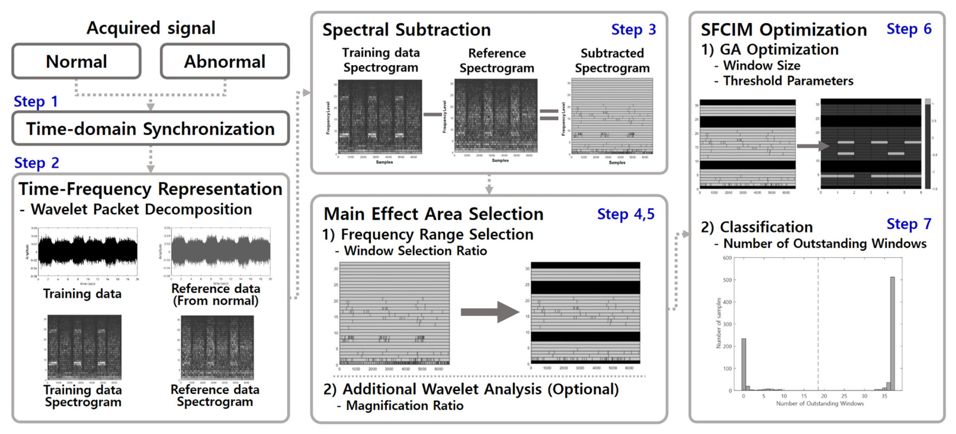
Fig.┬Ā2
Feature selection based dominant frequency range selection 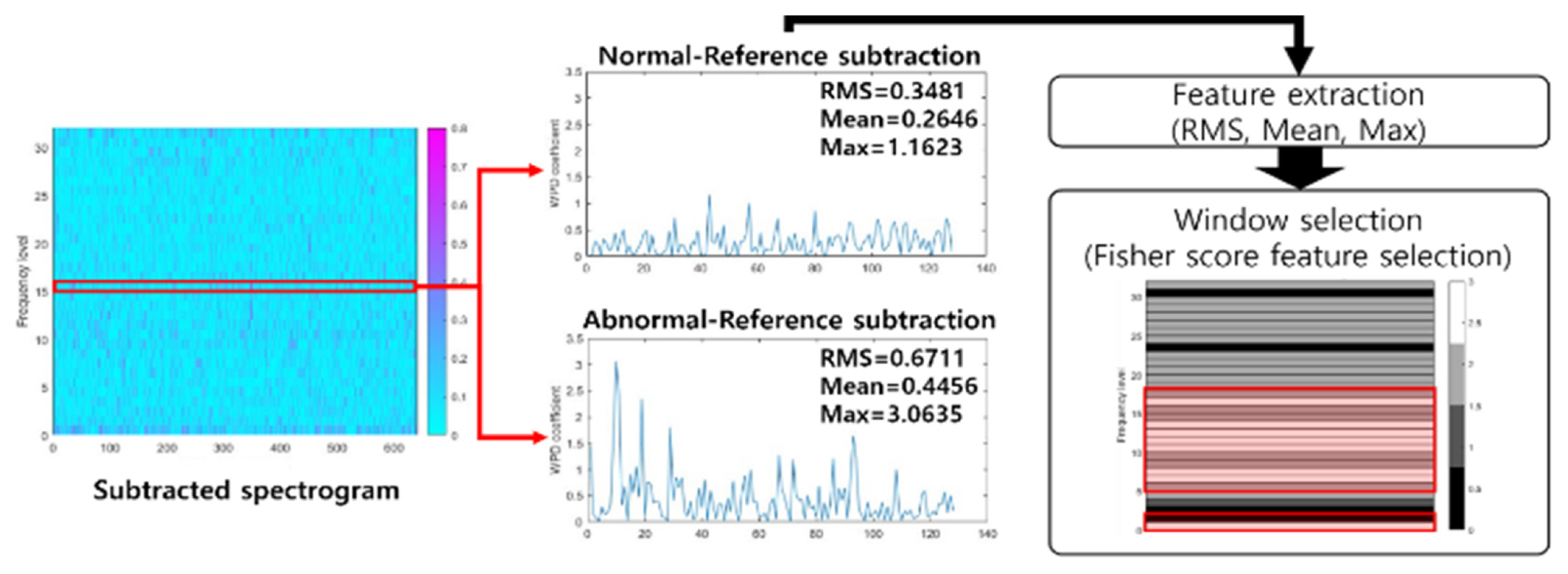
Fig.┬Ā3
Problem formulation of SFCIM optimization 
Fig.┬Ā4
Optimization variables for SFCIM optimization process 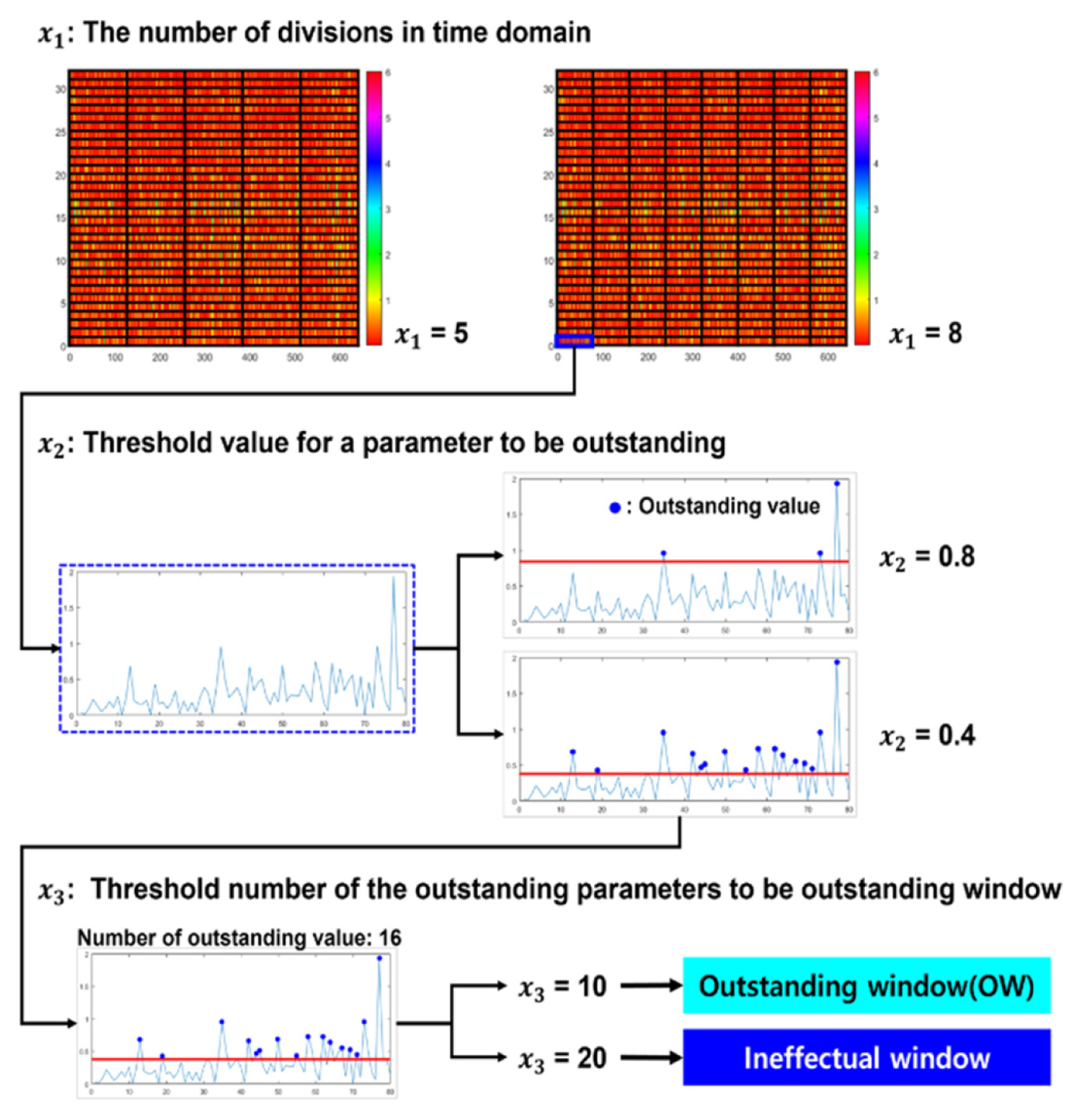
Fig.┬Ā5
Bearing test rig setup scheme 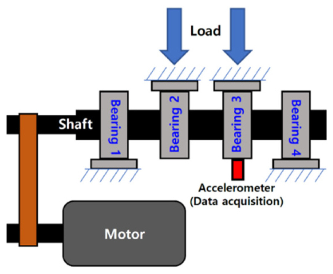
Fig.┬Ā6
Examples of subtracted spectrograms of (a) N-R and (b) A-R 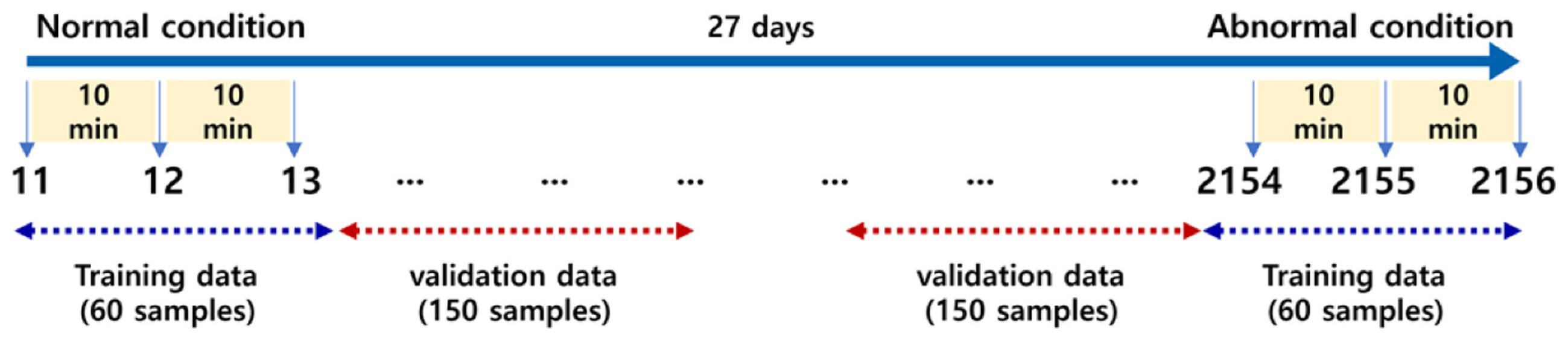
Fig.┬Ā7
Examples of subtracted spectrograms of (a) N-R and (b) A-R 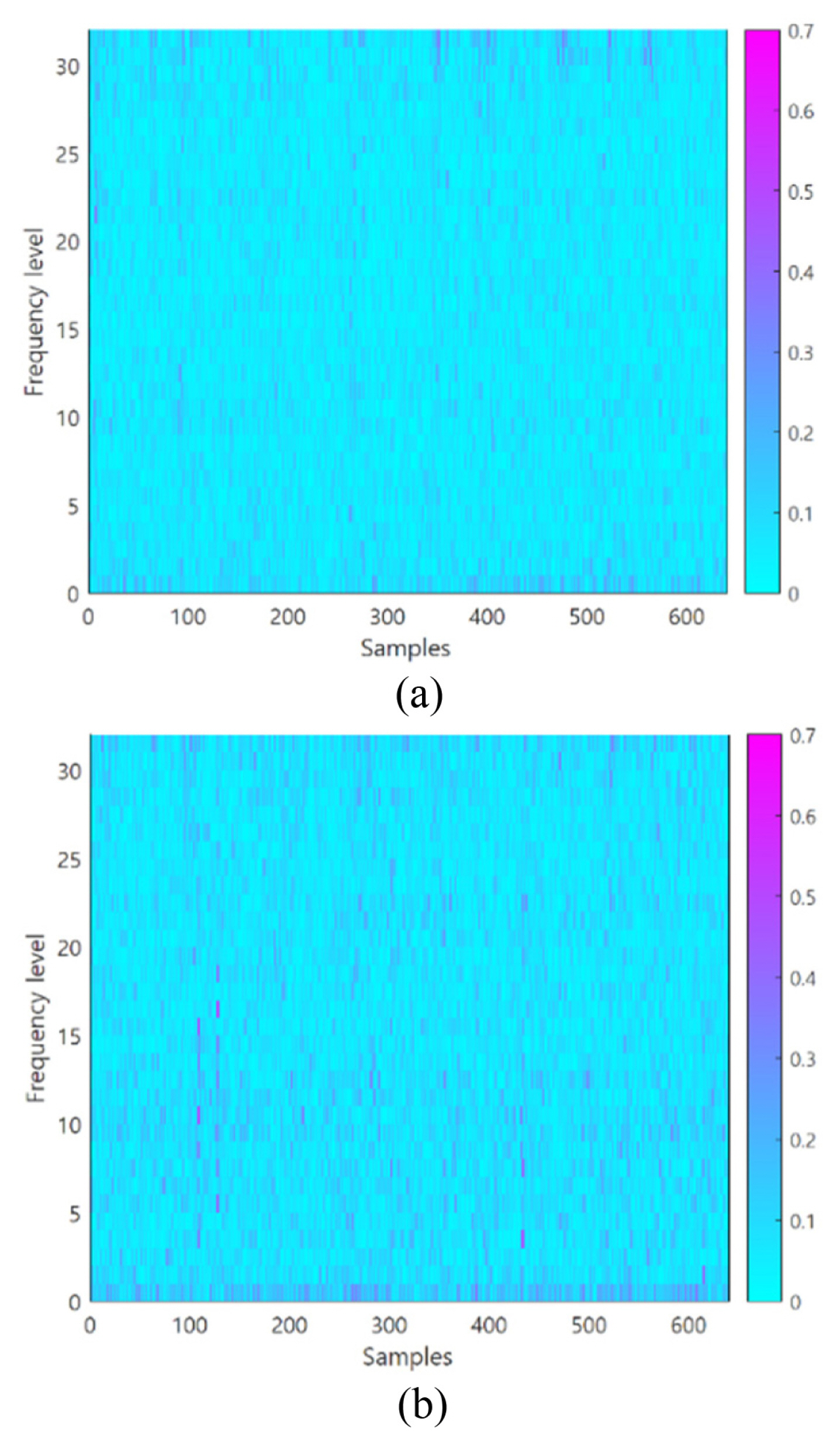
Fig.┬Ā8
(a) SFCIM for N-R vs. A-R, (b) Selected OWs in SFCIM 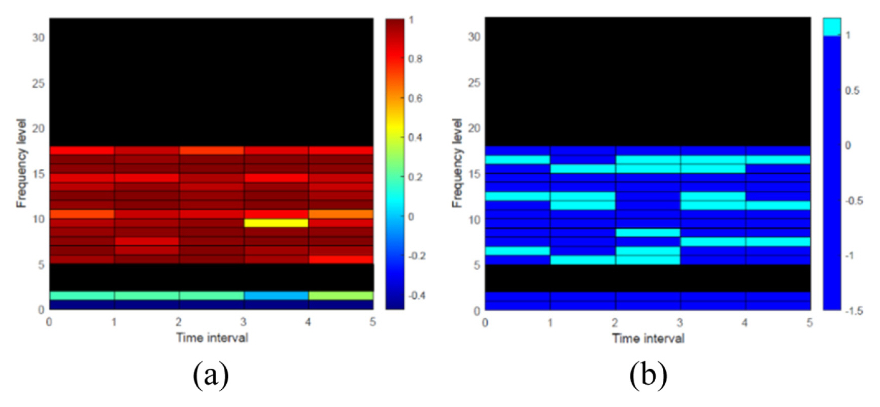
Fig.┬Ā9
Coefficients of the example OW 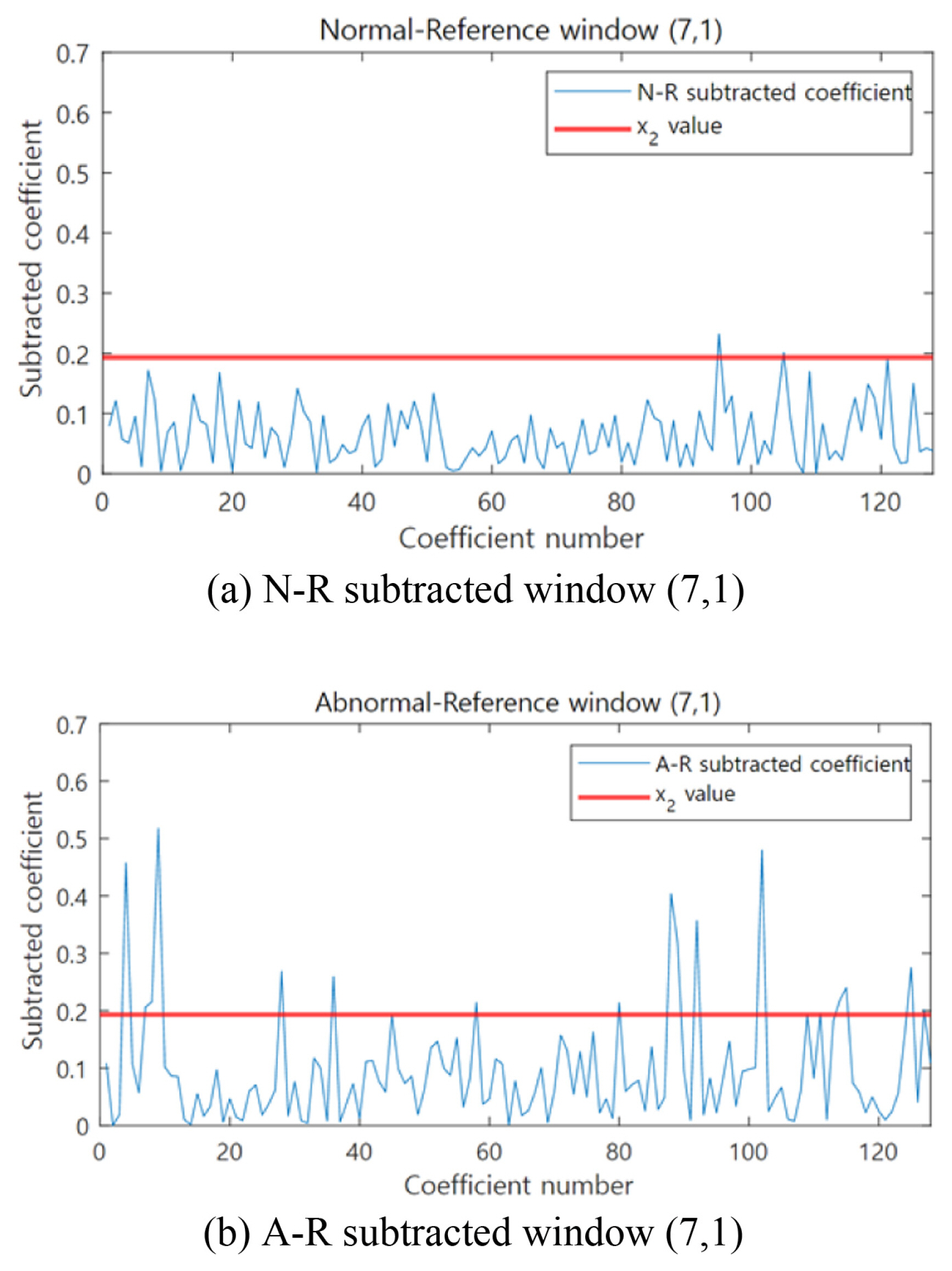
Fig.┬Ā10
Number of OWs for classification (IMS data) 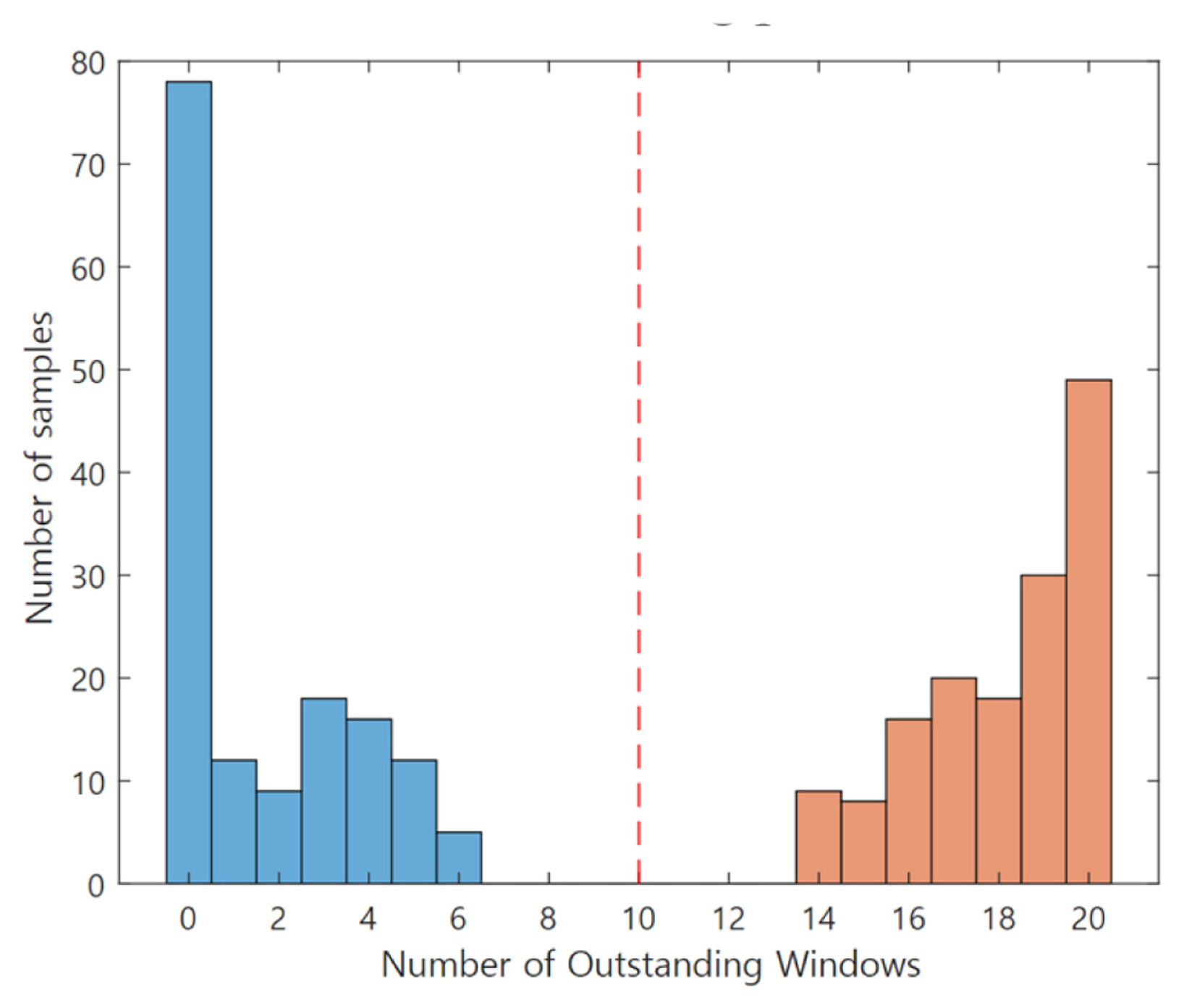
Fig.┬Ā11
Experimental setup for the pitting fault on the industrial robot 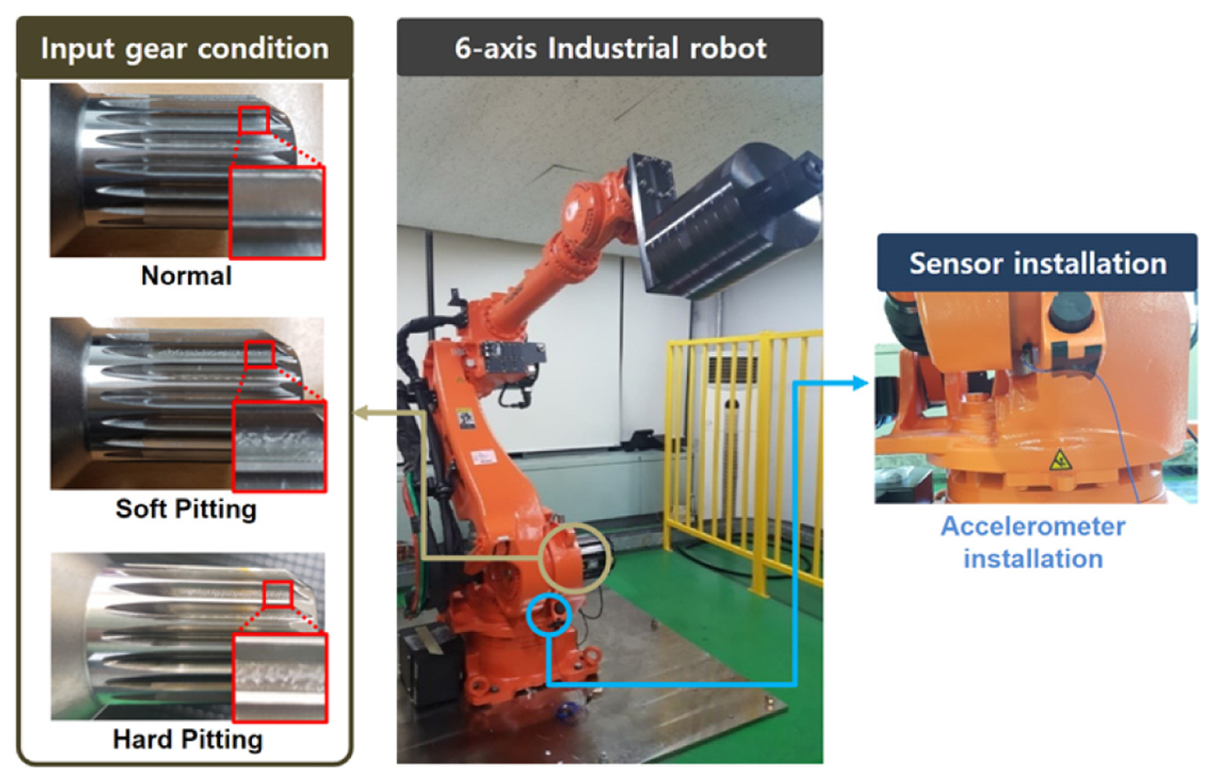
Fig.┬Ā12
Flow chart of the two-stage fault classification process 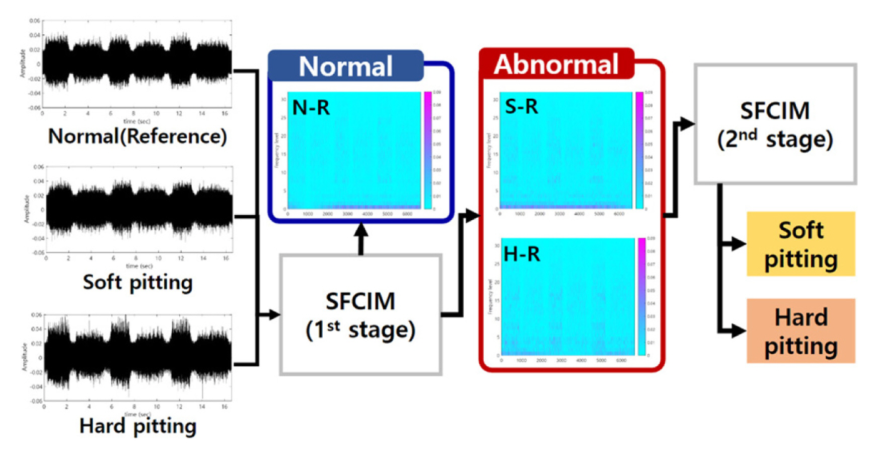
Fig.┬Ā13
Subtracted spectrograms: (a) N-R (b) S-R (c) H-R 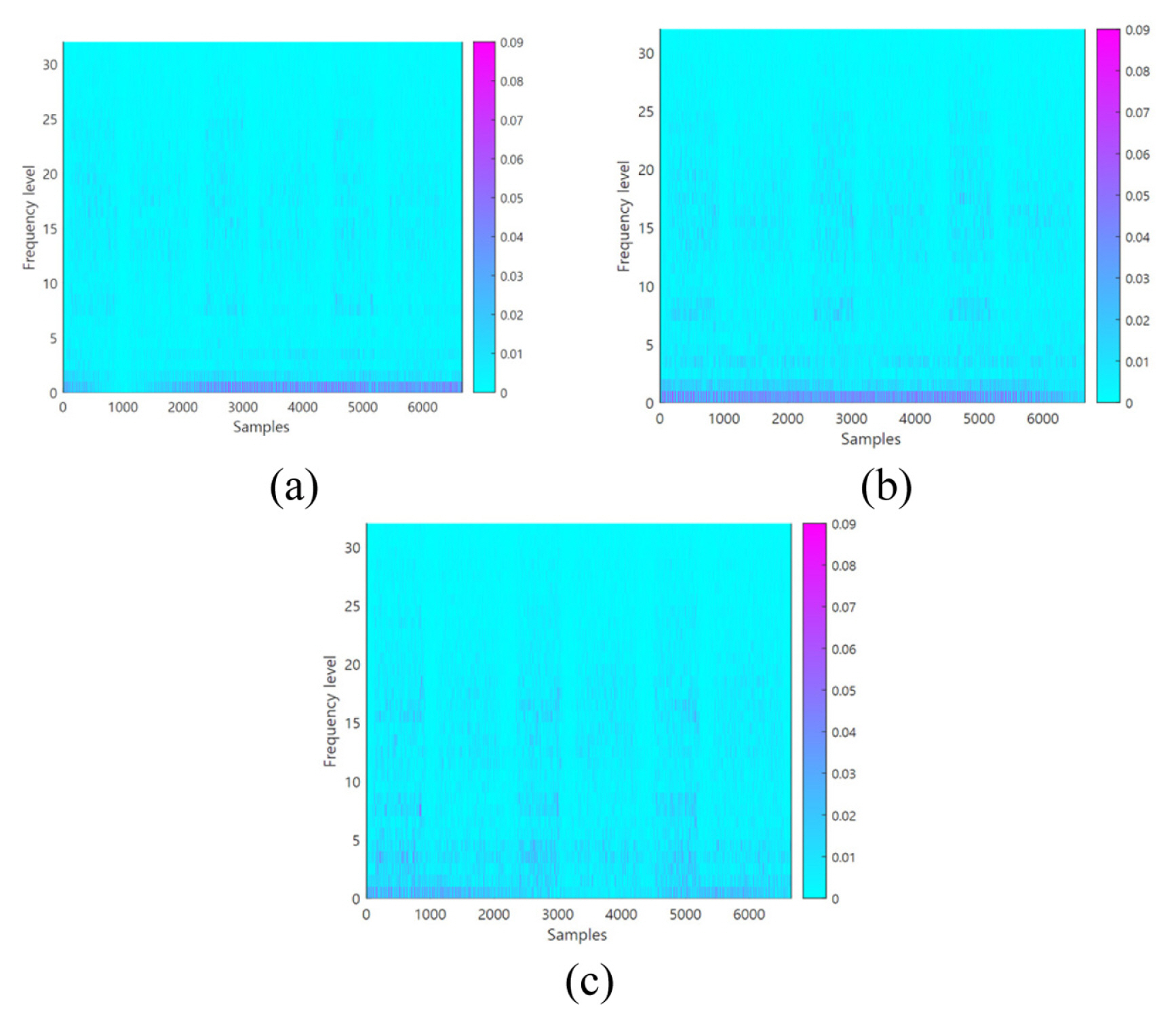
Fig.┬Ā14
SFCIM for fault classification and selected OWs 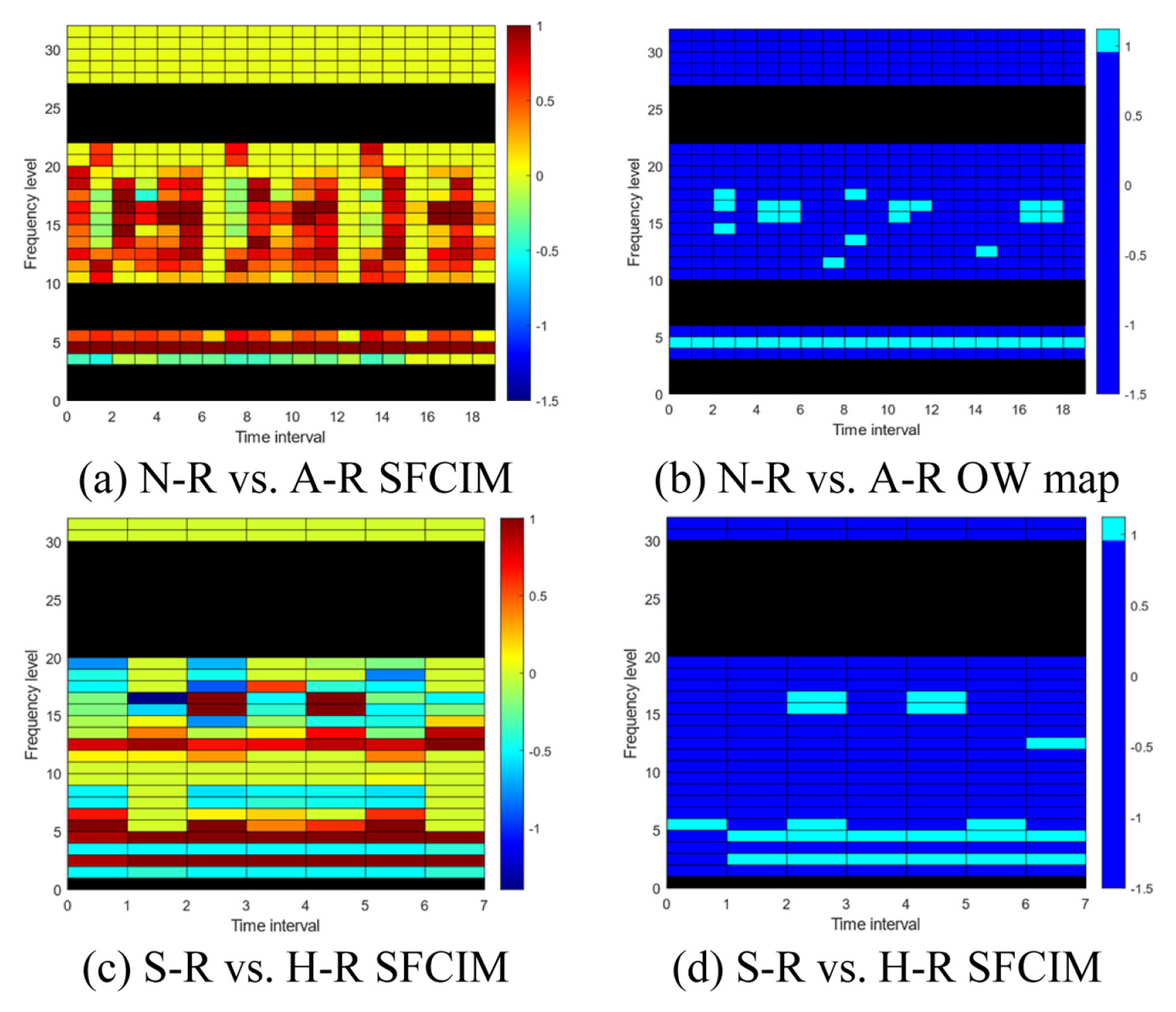
Fig.┬Ā15
Number of OWs for classification (Industrial robot input gear) 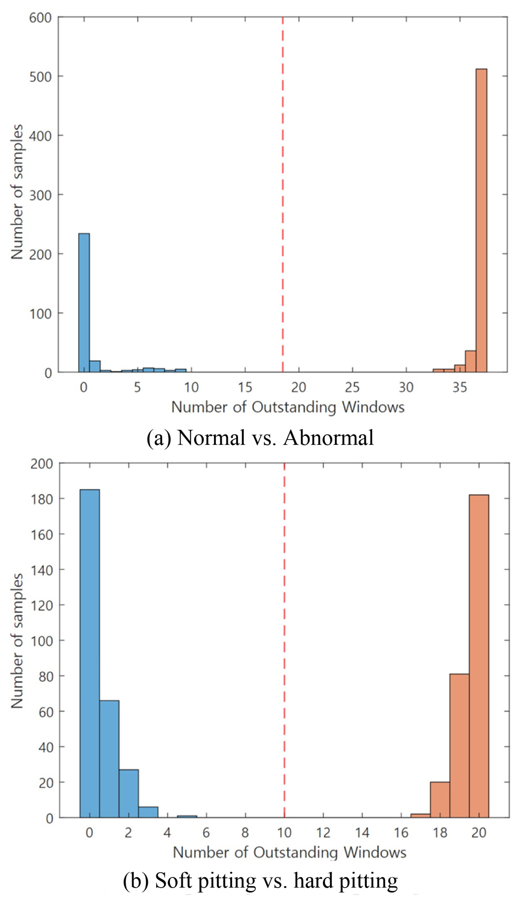
Fig.┬Ā16
Scheme of the experimental setup for grease level monitoring 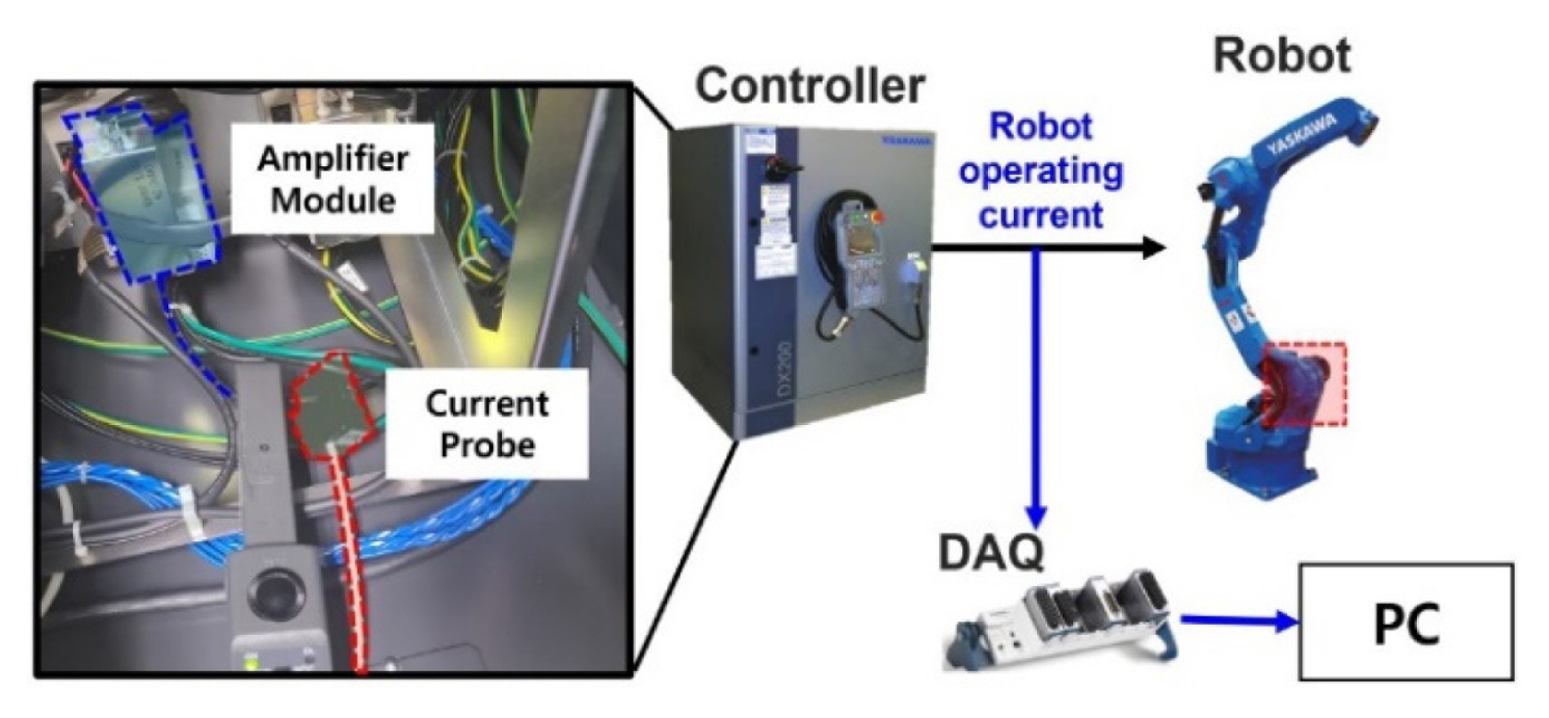
Fig.┬Ā17
Examples of subtracted spectrograms of (a) N-R and (b) A-R 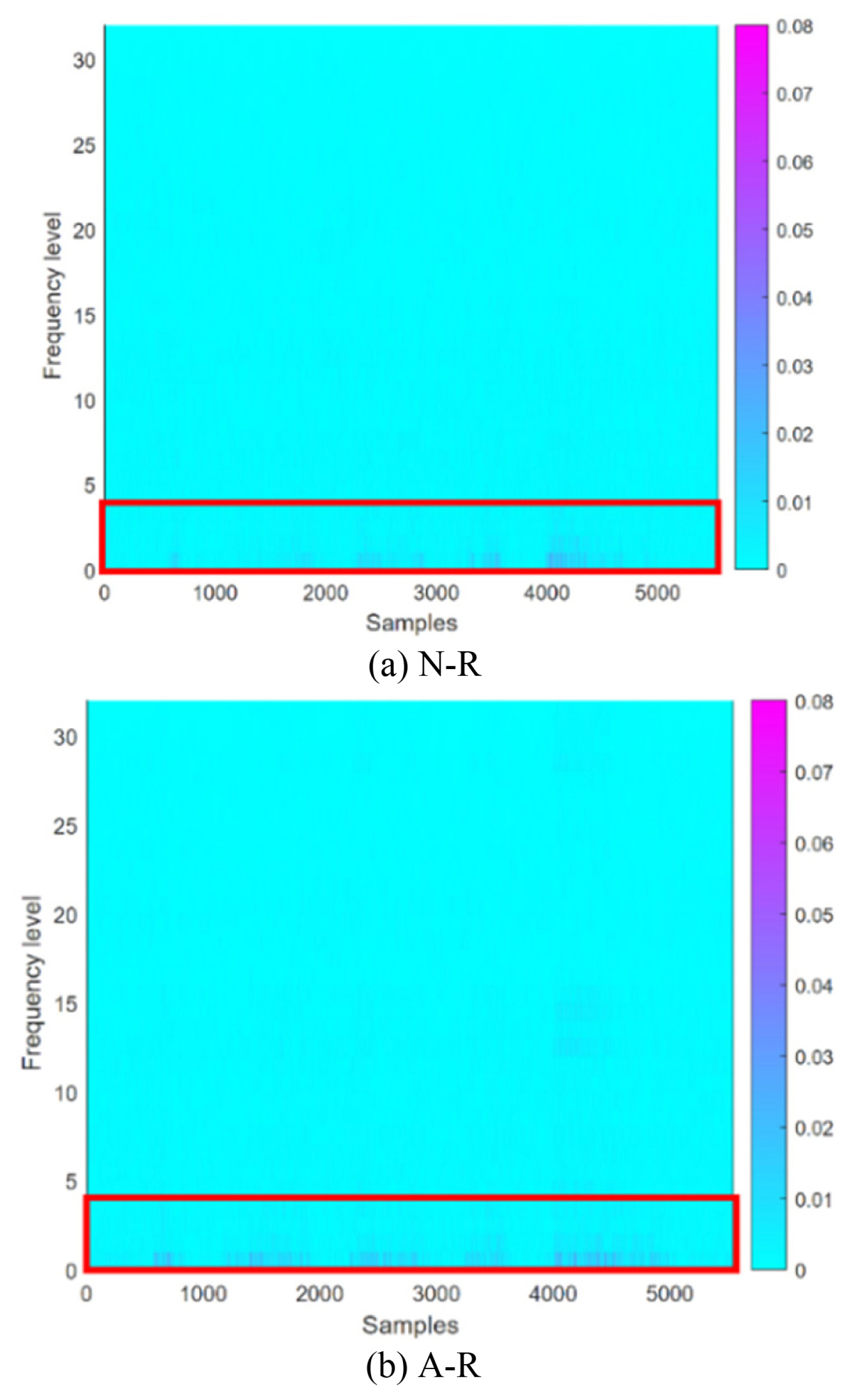
Fig.┬Ā18
Selected OWs in SFCIM for N-R vs. A-R 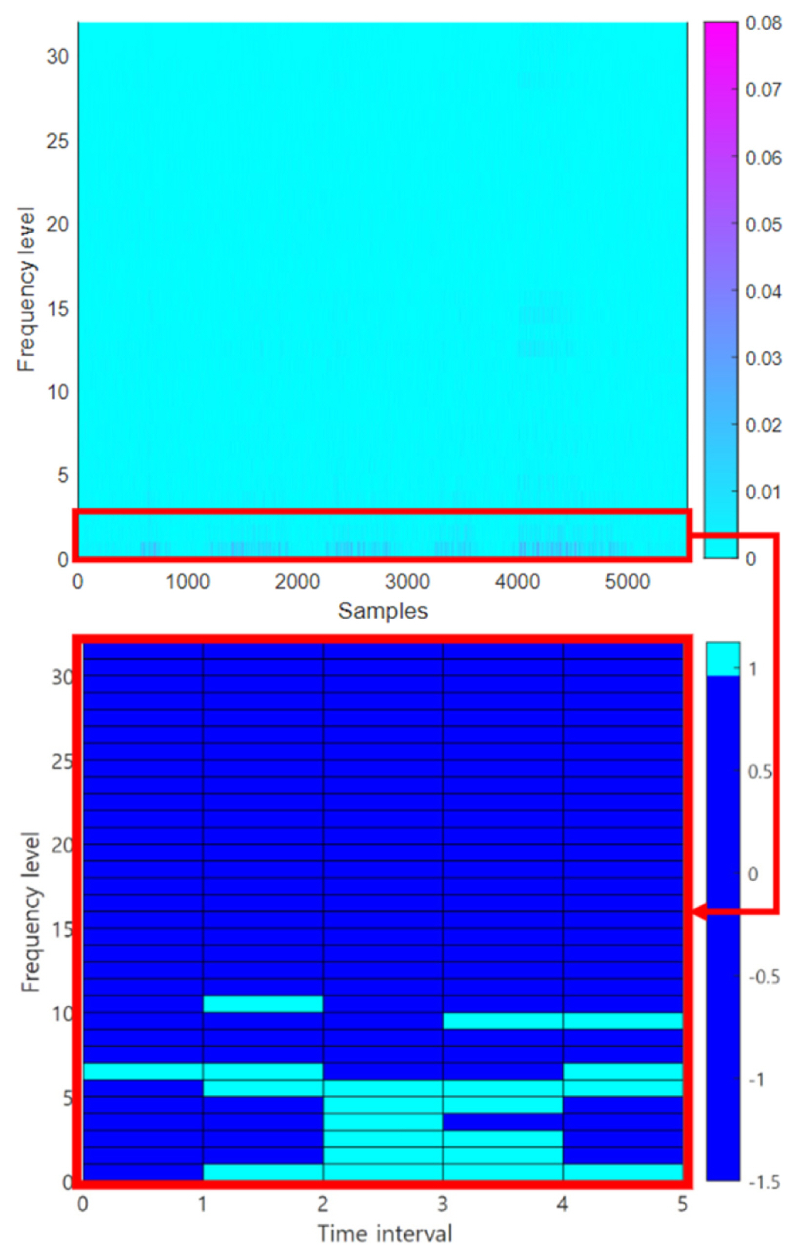
Fig.┬Ā19
Number of OWs for classification (Grease level detection) 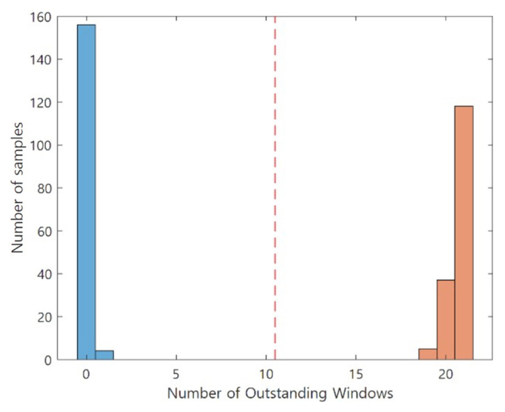
Table┬Ā1
Defined and optimized design variables (IMS dataset)
|
SFCIM parameters |
IMS data (N-R vs. A-R) |
|
WSR
|
0.67 |
|
Rc
|
0.99 |
|
Cp
|
1.5 |
|
x1
|
5 |
|
x2
|
0.1932 |
|
x3
|
7 |
Table┬Ā2
Confusion matrix of the validation result (IMS dataset)
|
Validation set result |
Ground truth |
|
Normal |
Normal |
|
Classification result (SFCIM) |
Normal |
150 |
0 |
|
Abnormal |
0 |
150 |
Table┬Ā3
Defined and optimized design variables (Industrial robot gear)
|
SFCIM parameters |
N-R vs. A-R (1st stage) |
S-R vs. H-R (2nd stage) |
|
WSR
|
0.67 |
0.67 |
|
Rc
|
0.95 |
0.95 |
|
Cp
|
1.5 |
1.5 |
|
x1
|
19 |
7 |
|
x2
|
0.0089 |
0.0224 |
|
x3
|
49 |
9 |
Table┬Ā4
Confusion matrix of the validation result (Gear pitting)
|
Validation set result |
Ground truth |
|
NC |
SP |
HP |
|
Classification result (SFCIM) |
NC |
285 |
0 |
0 |
|
SP |
0 |
285 |
0 |
|
HP |
0 |
0 |
285 |
Table┬Ā5
Defined and optimized design variables (S-R vs. H-R)
|
SFCIM parameters |
S-R vs. H-R (2nd stage) |
|
WSR
|
0.16 |
|
MR
|
4 |
|
Rc
|
0.99 |
|
Cp
|
1.5 |
|
x1
|
5 |
|
x2
|
0.0527 |
|
x3
|
2 |
Table┬Ā6
Confusion matrix of the validation result (Grease level)
|
Validation set result |
Ground truth |
|
Normal |
Normal |
|
Classification result (SFCIM) |
Normal |
150 |
0 |
|
Abnormal |
0 |
150 |
Table┬Ā7
Model performance comparison with IMS dataset
|
Method |
Fault detection performance |
|
Accuracy [%] |
Sensitivity [%] |
Specificity [%] |
Precision [%] |
|
Adaptive 1D CNN |
95.7 |
93.5 |
97.3 |
97.2 |
|
2D CNN |
95.9 |
97.0 |
97.0 |
95.7 |
|
Feature + ANN |
84.2 |
81.8 |
87.6 |
89.1 |
|
SFCIM |
100 |
100 |
100 |
100 |
Table┬Ā8
Computational time comparison result (IMS dataset)
|
Process |
Computational time |
|
Proposed method (SFCIM) (sec) |
Previous method (CIM) (sec) |
|
WPD based TFR |
7.2 |
7.2 |
|
Frequency range selection |
5.6 |
N/A |
|
Map optimization |
73.4 |
128.9 |
|
Total |
86.2 |
136.1 |
References
1. Wang, X., Mao, D. & Li, X. (2021). Bearing fault diagnosis based on vibro-acoustic data fusion and 1D-CNN network. Measurement, 173, 108518.  2. Elforjani, M., & Mba, D. (2010). Accelerated natural fault diagnosis in slow speed bearings with Acoustic Emission. Engineering Fracture Mechanics, 77(1), 112ŌĆō127. 3. Widodo, A., Yang, B.-S., Gu, D.-S. & Choi, B.-K. (2009). Intelligent fault diagnosis system of induction motor based on transient current signal. Mechatronics, 19(5), 680ŌĆō689. 4. Peng, Y., Qiao, W., Cheng, F. & Qu, L. (2021). Wind turbine drivetrain gearbox fault diagnosis using information fusion on vibration and current signals. IEEE Transactions on Instrumentation and Measurement, 70, 1ŌĆō11.   5. Das, B., Pal, S. & Bag, S. (2017). Torque based defect detection and weld quality modelling in friction stir welding process. Journal of Manufacturing Processes, 27, 8ŌĆō17. 6. Han, L., & Qi, H. (2019). Dynamics responses analysis in frequency domain of helical gear pair under multi-fault conditions. Journal of Mechanical Science and Technology, 33(11), 5117ŌĆō5127. 7. Masmoudi, M. L., Etien, E., Moreau, S. & Sakout, A. (2017). Single point bearing fault diagnosis using simplified frequency model. Electrical Engineering, 99(1), 455ŌĆō465. 8. Gao, Z., Cecati, C. & Ding, S. X. (2015). A survey of fault diagnosis and fault-tolerant techniques-Part I: Fault diagnosis with model-based and signal-based approaches. IEEE Transactions on Industrial Electronics, 62(6), 3757ŌĆō3767. 9. Gao, Z., Cecati, C. & Ding, S. (2015). A survey of fault diagnosis and fault-tolerant techniques Part II: Fault diagnosis with knowledge-based and hybrid/active approaches. IEEE Transactions on Industrial Electronics, 62(6), 3768ŌĆō3774. 10. Li, R., Sopon, P. & He, D. (2012). Fault features extraction for bearing prognostics. Journal of Intelligent Manufacturing, 23(2), 313ŌĆō321. 11. Kong, Y., Wang, T. & Chu, F. (2019). Meshing frequency modulation assisted empirical wavelet transform for fault diagnosis of wind turbine planetary ring gear. Renewable Energy, 132, 1373ŌĆō1388. 12. Chen, C.-C., Liu, Z., Yang, G., Wu, C.-C. & Ye, Q. (2020). An Improved Fault Diagnosis Using 1D-Convolutional Neural Network Model. Electronics, 10(1), s. 59. 13. Zhang, Y., Xing, K., Bai, R., Sun, D. & Meng, Z. (2020). An enhanced convolutional neural network for bearing fault diagnosis based on time-Frequency image. Measurement, 157, 107667. 14. Papoulis, A. (1962). The fourier integral and its applications, 1st ed.. McGraw-Hill: New York.
15. Peng, Z., & Chu, F. (2004). Application of the wavelet transform in machine condition monitoring and fault diagnostics: A review with bibliography. Mechanical Systems and Signal Processing, 18(2), 199ŌĆō221. 16. Verstraete, D., Ferrada, A., Droguett, E. L., Meruane, V. & Modarres Enhancement of speech corrupted by acoustic noise M. (2017). Deep learning enabled fault diagnosis using time-frequency image analysis of rolling element bearings. Shock and Vibration, 2017, 1ŌĆō17. 17. Yen, G. G., & Lin, K.-C. (2000). Wavelet packet feature extraction for vibration monitoring. IEEE Transactions on Industrial Electronics, 47(3), 650ŌĆō667. 18. Berouti, M., Schwartz, R. & Makhoul, J. (1979). Enhancement of speech corrupted by acoustic noise. IEEE International Conference on Acoustics, Speech, and Signal Processing (pp. 208ŌĆō211. 19. Denda, Y., Nishiura, T.Kawahara, H. & Irino, T. (2004). Speech recognition with wavelet spectral subtraction in real noisy environment. In: Proceedings 7th International Conference on Signal Processing; pp 638ŌĆō641. 20. Bouchikhi, E. H. E., Choqueuse, V. & Benbouzid, M. E. H. (2013). Current frequency spectral subtraction and its contribution to induction machinesŌĆÖ bearings condition monitoring. IEEE Transactions on Energy Conversion, 28(1), 135ŌĆō144. 21. Li, J., Cheng, K., Wang, S., Morstatter, F., Trevino, R. P., Tang, J. & Liu, H. (2017). Feature selection: A data perspective. ACM Computing Surveys (CSUR), 50(6), 1ŌĆō45.
22. Qiu, H., Lee, J., Lin, J. & Yu, G. (2006). Wavelet filter-based weak signature detection method and its application on rolling element bearing prognostics. Journal of sound and vibration, 289(4ŌĆō5), 1066ŌĆō1090. 23. Tan, C. K., Irving, P. & Mba, D. (2007). A comparative experimental study on the diagnostic and prognostic capabilities of acoustics emission, vibration and spectrometric oil analysis for spur gears. Mechanical Systems and Signal Processing, 21(1), 208ŌĆō233. 28. Ince, T., Kiranyaz, S., Eren, L., Askar, M. & Gabbouj, M. (2016). Real-time motor fault detection by 1-D convolutional neural networks. IEEE Transactions on Industrial Electronics, 63(11), 7067ŌĆō7075. 29. Peng, H., Long, F. & Ding, C. (2005). Feature selection based on mutual information criteria of max-dependency, max-relevance, and min-redundancy. IEEE Transactions on Pattern Analysis and Machine Intelligence, 27(8), 1226ŌĆō1238. 30. Aha, D. W., & Bankert, R. L. (1995). A comparative evaluation of sequential feature selection algorithms. In: Pre-Proceedings of the Fifth International Workshop on Artificial Intelligence and Statistics; pp 1ŌĆō7. 31. Van Stralen, K. J., Stel, V. S., Reitsma, J. B., Dekker, F. W., Zoccali, C. & Jager, K. J. (2009). Diagnostic methods I: sensitivity, specificity, and other measures of accuracy. Kidney International, 75(12), 1257ŌĆō1263. 32. Huh, J., Pham Van, H., Han, S., Choi, H. J. & Choi, S. K. (2019). A data-driven approach for the diagnosis of mechanical systems using trained subtracted signal spectrograms. Sensors, 19(5), 1055. 
Biography
Seungyon Cho received bachelorŌĆÖs and masterŌĆÖs degree from the School of Mechanical Engineering, Chung-Ang University, Seoul, Korea, in 2022. His academic interests include signal processing, mechanical system fault diagnosis, prognostics and health management, and machine learning.
Biography
Hea-Ryeon Seo received bachelorŌĆÖs degree from the School of Mechanical Engineering, Chung-Ang University, Seoul, Korea, in 2022. She is currently a graduate student in the School of Mechanical Engineering, Chung-Ang University (CAU). Her academic interests include mechanical system monitoring, fault diagnosis, prognostics and health management, and machine learning.
Biography
Geonhwi Lee is currently a B.S. candidate in the School of Mechanical Engineering, Chung-Ang University (CAU). His academic interests include mechanical system monitoring, prognostics and health management, signal processing, and machine learning.
Biography
Seung-Kyum Choi is an Associate Professor in School of Mechanical Engineering at Georgia Institute of Technology. Dr. ChoiŌĆÖs research interests include structural reliability, probabilistic mechanics, statistical approaches to design of structural systems, multidisciplinary design optimization, and information engineering for complex engineered systems. He served as Invited Guest Editors for Journal of Engineering Design and Journal of Electronic Materials. He also served as a Chair and Session Organizer at national conferences of AIAA, SDM, MDO, NDA and ASME/IDETC, in addition to being an invited member of the AIAA Non-Deterministic Technical Committee. Since 2017, Dr. Choi is currently appointed the Director of Center for Additive Manufacturing Systems (CAMS), where he has responsibilities for developing research and educational programs in additive manufacturing.
Biography
Hae-Jin Choi received M.S. and Ph.D. degrees in Mechanical Engineering from the Georgia Institute of Technology (Georgia Tech), Atlanta, GA, USA, in 2001 and 2005, respectively. He was an Assistant Professor at Nanyang Technological University, Singapore. He was also a Postdoctoral Fellow at the GWW School of Mechanical Engineering, Georgia Tech. He is currently a Professor at the School of Mechanical Engineering, Chung-Ang University, Seoul, Korea. His research interests include fault diagnosis, prognostics and health management, machine learning, simulation-based design optimization, management of uncertainty, and integrated materials and products design.
|
|
| TOOLS |
|
|
|
|
|
|
|
|
|
|
|
|
|
|
METRICS

|
|
|
|
|
|

 E-mail
 Print
Print facebook
 twitter
 Linkedin
 google+


 PDF Links
 PubReader
 Full text via DOI
 Download Citation
  CrossRef TDM


